Plan, Activity, and Intent Recognition: Theory and Practice, FIRST EDITION (2014)

Part I. Plan and Goal Recognition

Chapter 4. Keyhole Adversarial Plan Recognition for Recognition of Suspicious and Anomalous Behavior

Dorit Avrahami-Zilberbrand and Gal A. Kaminka, Bar Ilan University, Ramat Gan, Israel

Abstract

Adversarial plan recognition is the use of plan recognition in settings where the observed agent is an adversary, having plans or goals that oppose those of the observer. It is one of the key application areas of plan-recognition techniques. There are two approaches to adversarial plan recognition. The first is suspicious activity recognition; that is, directly recognizing plans, activities, and behaviors that are known to be suspect (e.g., carrying a suitcase, then leaving it behind in a crowded area). The second is anomalous activity recognition in which we indirectly recognize suspect behavior by first ruling out normal, nonsuspect behaviors as explanations for the observations. Different challenges are raised in pursuing these two approaches.

In this chapter, we discuss a set of efficient plan-recognition algorithms that are capable of handling the variety of challenges required of realistic adversarial plan-recognition tasks. We describe an efficient hybrid adversarial plan-recognition system composed of two processes: a plan recognizer capable of efficiently detecting anomalous behavior, and a utility-based plan recognizer incorporating the observer’s own biases—in the form of a utility function—into the recognition process. This allows choosing recognition hypotheses based on their expected cost to the observer. These two components form a highly efficient adversarial plan recognizer capable of recognizing abnormal and potentially dangerous activities. We evaluate the system with extensive experiments using real-world and simulated activity data from a variety of sources.

Keywords

Adversarial plan recognition

Utility-based plan recognition

Anomalous plan recognition

Suspicious plan recognition

Acknowledgments

We thank the anonymous reviewers and this book’s editors for their very valuable and detailed comments on early drafts of this chapter. This research was carried out with partial support from the Israeli Ministry of Commerce’s AVNET Consortium and the Israel Science Foundation, Grant #1511/12. As always, thanks to K. Ushi.

4.1 Introduction

Adversarial plan recognition is the use of plan recognition in settings where the observed agent is considered a potential adversary, having plans or goals that oppose those of the observer. The objective of adversarial plan recognition is to identify behavior that is potentially harmful, differentiating it from nonadversarial behavior, in time for the observer to decide on a reaction. Applications of adversarial plan recognition include computer intrusion detection [23], virtual training environments [56], in-office visual surveillance [10], and detection of anomalous activities [17,45,59]. Adversarial plan recognition faces several inherent challenges:

• First, often there are limited data from which to construct a plan library of the adversary’s behavior. Unlike with most plan-recognition settings, we cannot assume knowledge of the complete set of plans an adversary may pursue. Thus, an adversarial plan-recognition system has to recognize anomalous plans—plans that are characterized simply by the fact that they are not known to the observing agent.

• Second, most nonadversarial plan-recognition systems ignore the expected impact of the explanations they generate on the observer. They generate a list of recognition hypotheses (typically ranked by decreasing likelihood). It is up to the observer’s decision-making component to examine the hypotheses and draw a conclusion leading to taking action. But often adversarial plan hypotheses have low likelihoods because of their rarity. Thus, they must either be ignored for being too unlikely or they must be considered together with many other low-likelihood hypotheses, which may lead to many false positives.

For instance, suppose we observe a rare sequence of Unix commands that can be explained for some plan or for a more common plan . Most plan-recognition systems will prefer the most likely hypothesis and ignore . Yet, if the risk of for the observer is high (e.g., if is a plan to take down the computer system), then that hypothesis should be preferred when trying to recognize suspicious behavior. If implies low risk (even if the observed sequence is malicious), or if the goal is not to recognize suspicious behavior, then may be a better hypothesis.

This chapter describes a comprehensive system for adversarial plan recognition. The system is composed of a hybrid plan recognizer: A symbolic recognition system, Symbolic Behavior Recognition (SBR) [3,4], is used to detect anomalous plans. Recognized nonanomalous plans are fed into an efficient utility-based plan-recognition (UPR) system [5], which reasons about the expected cost of hypotheses, recognizing suspicious plans even if their probability is low.

We evaluate the two components in extensive experiments using real-world and simulated activity data from a variety of sources. We show that the techniques are able to detect both anomalous and suspicious behavior while providing high levels of precision and recall (i.e., small numbers of false positives and false negatives).

4.2 Background: Adversarial Plan Recognition

Plan recognition is the task of inferring the intentions, plans, and/or goals of an agent based on observations of its actions and observable features. Other parts of this book provide an extensive survey of past and current approaches to plan recognition. We focus here on adversarial settings in which plan recognition is used to recognize plans, activities, or intentions of an adversary.

Applications of plan recognition to surveillance in particular, and adversarial plan recognition in general, began to appear shortly after the introduction of the basic probabilistic recognition methods (e.g., Hilary and Shaogang [26]) and continue to this day in studies done by various authors [10,15,17,23,38,40,45,59]. We survey recent efforts in the following.

We limit ourselves to keyhole recognition, where the assumption is that the adversary is either not aware that it is being observed or does not care. Toward the end of this section, we discuss relaxing this assumption (i.e., allowing intended recognition, where the observed adversary possibly modifies its behavior because it knows it is being observed).

One key approach to adversarial plan recognition is anomalous plan recognition, based on anomaly detection (i.e., recognition of what is not normal). Here, the plan library is used in an inverse fashion; it is limited to accounting only for normal behavior. When a plan recognizer is unable to match observations against the library (or generates hypotheses with very low likelihood), an anomaly is announced.

The second key approach to adversarial plan recognition is suspicious plan recognition, based on directly detecting threatening plans or behavior. It operates under the assumption that a plan library is available that accounts for adversarial behavior; thus, recognition of hypotheses implying such behavior is treated no differently than recognition of hypotheses implying normal activity.

In both approaches, there is an assumption that the plan library is complete, in that it accounts for the full repertoire of expected normal behavior (in anomalous plan recognition) or adversarial behavior (in suspicious plan recognition). Likewise, a full set of observable features can be used for either approach: not only the type of observed action but also its duration and its effects; not only the identity of the agent being observed but also observable features that mark it in the environment (i.e., its velocity and heading, its visual appearance, etc.).

Superficially, therefore, a plan-recognition system intended for one approach is just as capable of being used for the other, as long as an appropriate plan library is used. However, this is not true in practice, because different approaches raise different challenges.

4.2.1 Different Queries

Fundamentally, the two approaches answer different queries about the observed agent’s behavior.

The main query that an anomalous behavior-recognition system has to answer is a set membership query: “Is the observed behavior explained by the plan library?” If so, then no anomaly is declared. If not, then an anomaly is found. Thus, the relative likelihood of the hypothesized recognized plan, with respect to other hypotheses, is not important.¹

In contrast, the main query that a suspicious behavior-recognition system has to answer is the current state query: “What is the preferred explanation for the observations at this point?” We use the term preferred because there are different ways of ranking plan-recognition hypotheses. The most popular one relies on probability theory to rank hypotheses based on their likelihood. But as we discuss later, this is only one way to rank hypotheses.

4.2.2 Origins of the Plan Library

The construction of a plan library for the two approaches, presumably by human experts or automated means, is based on knowledge sources that have different characteristics.

In many adversarial settings, knowledge of the adversarial behavior is clearly available. For instance, in applications of plan recognition in recognizing a fight between a small number of people, it is possible to imagine a specific set of recognition rules (e.g., accelerated limb motions, breaking of personal distances). If such knowledge exists, suspicious behavior recognition is more easily used.

However, in some settings, knowledge of specific adversarial plans is lacking and examples are rare. For instance, in surveillance for terrorist attacks in airport terminals, there are very few recorded examples, and certainly we cannot easily enumerate all possible ways in which the adversary might act prior to an attack. Here, the use of anomalous behavior recognition is more natural.

4.2.3 The Outcome from the Decision-Making Perspective

A challenge related to the different queries is the use of the output from the plan-recognition module as a basis for decision making. In suspicious plan recognition, the greater the match between the observations and the plan library (as measured by likelihood or another means), the greater the confidence in categorizing the behavior as suspicious. This can be used by a decision-making module to respond appropriately to different levels of suspiciousness (e.g., by actively taking actions to differentiate hypotheses or directly counter the implied threat).

But in the anomalous behavior-recognition case, the opposite is true. The weaker the match between the observations and the plan library, the greater the implied confidence in the anomaly. However, because in this case a sequence of observations is considered anomalous when it does not exist in the plan library, there is no universally accepted method for assessing confidence in the outcome. In other words, there is no universally correct method for measuring the degree to which the observations do not match the plan library.

We first discuss existing work using anomalous plan recognition. This approach has connections to machine learning (e.g., one-class learning for security) and monitoring (e.g., fault detection and diagnosis). The literature on anomaly detection within these areas is vast. However, much of it is only superficially related, in the sense that the overall goals may be the same, but the application domains give rise to methods that are very data-oriented yet require little or no treatment of hierarchical states, interleaved activities, or future intentions. For instance, fingerprinting users from their characteristic behavior (e.g., see Lane and Brodley [37]) is a related task, but the focus is on supervised machine learning of mouse and keyboard events. Similarly, we will not address here related work done by various authors on anomaly detection in data signals. (e.g., [1,16,35]).

Within plan-recognition literature, Xiang and Gong [60] adopted dynamic Bayesian networks (DBNs) to model normal patterns of activity captured on video. An activity is identified as abnormal if the likelihood of it being generated by normal models is less then a threshold. Duong et al. [17] use Switching Semi-Markov Models to represent user activities that have a known duration (so an anomaly is detected if actions’ durations deviate from normal). Marhasev et al. [43] look at low-likelihood hypotheses based on both duration and state in the context of a clinical diagnosis task.

Yin et al. [62] present a two-phase approach to detect anomalous behavior based on wireless sensors attached to the human body. This approach first uses Support Vector Machines (SVMs) that filter out the activities with a high probability of being normal, then derives from these an anomalous activity model. Here also the model is learned based on normal activities.

One key issue with all of these investigations is that they spend computational time on probabilistic reasoning that might not be necessary for a membership query. In contrast, we advocate an approach that uses symbolic behavior recognition, which can answer the membership query much more efficiently.

In particular, the SBR algorithms [3,4] advocated in this chapter provide extremely efficient membership query responses at the expense of recognition accuracy (since they cannot rank hypotheses based on likelihood). The SBR algorithms are most related to symbolic plan-recognition algorithms used to identify failures in teamwork. RESL [34], and later YOYO [30], are symbolic recognition algorithms for detecting disagreements among team members. Both RESL and YOYO exploit knowledge of the social structures of the team (called team hierarchy) to efficiently recognize splits in teams, where an agent is executing a different plan than agreed on with the rest of its team. Disagreements are therefore treated as recognition failures. Both algorithms ignore observation history in current state hypotheses in contrast to SBR. Moreover, these algorithms do not account for complex temporal reasoning (i.e., duration and interleaving), while SBR algorithms do.

We now turn to discussing work in suspicious behavior recognition. It operates under the assumption that the plan library directly covers the adversarial behavior to be recognized. Thus, recognition of hypotheses implying such behavior is treated no differently than recognition of hypotheses implying normal activity. Examples include systems that encode possible attacks in an intrusion-detection system, trying to predict whether an attack is performed [23]; systems that focus on recognizing specific suspicious behaviors in train stations [15] (e.g., fighting); systems with an a priori set of attack templates [29] that are compared with observations to infer whether a particular terrorist attack matches one or more templates; and models with representations of human activities based on tracked trajectories—for example, see Niu et al. [45].

Most suspicious behavior-recognition systems use probabilistic plan-recognition approaches. These focus on determining the most likely hypothesis, or set of hypotheses, as to the current and/or past states of the agent. Previous work in this area has focused on using specialized structures and techniques that allow more efficient recognition or more expressive forms of plan recognition.

Some of the early work applying plan recognition to visual surveillance applied belief (Bayesian) networks (e.g., see Hilary and Shaogang [26] and Hongeng et al. [27]). However, given the known computational hardness of exact and approximate reasoning in general belief networks [14] and general dynamic belief networks [8,36], more efficient models were needed. These typically trade expressiveness for runtime (e.g., by introducing a Markov assumption into the models).

Indeed, Hidden Markov Models (HMMs) and extensions have been explored extensively for plan recognition. These are special cases of dynamic belief networks, with much improved inference runtime (typically, polynomial), at the cost of introducing a Markovian assumption and restricting the set of variables. HMMs are widely used for recognition of simple activities (e.g., see Starner and Pentland [52] and Yamato et al. [61]). However, they do not allow for complex activities (e.g., interacting agents, hierarchical decomposition of the activities, or explicit temporal dependencies). Coupled HMMs [9] and Factorial HMMs [25] are extensions of the HMM with multiple hidden interacting chains (e.g., for modeling interactions between observed agents).

AHMMs [11], HHMMs [18], and Layered HMMs [47] are capable of handling activities that have hierarchical structures. These models are used in activity-recognition applications (e.g., learning and detecting activities from movement trajectories [44]) and inferring user’s daily movements from raw GPS sensor data [38]. Hidden Semi-Markov Models (HSMMs) allow probabilistic constraints over the duration of plans [17]. Extensions to these can model dependencies on state durations [43]. More recent work has continued developing methods for greater expressiveness without sacrificing tractability. For example, Blaylock and Allen [7] provided a novel HMM-based model that allows efficient exact reasoning about hierarchical goals. Hu and Yang [28] model interacting and concurrent goals.

Recent work has moved beyond dynamic belief networks and Markov models to use conditional random fields [57], which allow for greater expressiveness. Bui et al. [12] introduce a Hidden Permutation model that can learn the partial ordering constraints in location-based activity recognition. There are also approaches to plan recognition based on parsing, in particular using probabilistic grammars, which allow for efficient exact inference (e.g., see the works of several authors [19–21,50,51]).

The key challenge to the use of probabilistic recognizers in suspicious behavior recognition is that most often adversarial behavior is not likely, typically because it is rare. Given a specific sequence of observations, if the adversarial hypothesis is the only explanation, then obviously it would be selected. But generally in plan recognition, there would be multiple hypotheses that match the observations and that have to be ranked in some fashion. In this general case, preferring the most likely hypothesis often means preferring the more common explanation rather than the rare explanation signifying adversarial intent.

In other words, the posterior likelihood of a hypothesis signifying adversarial behavior is very often low, given the observations. In the general case, it would be one hypothesis out of many. This leads to either of two cases: the observer has to always consider low-likelihood hypotheses (leading to many false alarms, i.e., false positives) or the observer sets a high threshold for likelihood, in which case she risks disregarding a suspicious behavior.

To address this, we posit that a system for suspicious plan recognition needs to reason about the expected cost to the observer, given that a hypothesis is correct. In other words, we argue that the observer ranks hypotheses based on their expected cost to itself rather than just based on their likelihood. This way, a low-likelihood hypothesis, which, if true, would signify large costs, may be preferred over a more likely hypothesis, which implies no risk. Put more generally, our work differs significantly from probabilistic approaches because we advocate reasoning about the expected utility of hypotheses rather than simply their likelihoods.

Essentially every probabilistic plan-recognition system can be used as the basis for expected cost computations. This can be done by taking the entire (ranked) set of hypotheses from the probabilistic recognizers and then externally associating each with costs to compute expected costs. Computationally, this can be very expensive because in addition to the plan-recognition computation, there would be more external computation of the expected costs. Note that the entire set of hypotheses must be processed, as a low-likelihood hypothesis (ranked low by the probabilistic recognizer) may end up implying a high expected utility.

The key to efficient computation of plan-recognition hypotheses, ranked by their expected costs, is the folding of the expected cost computation into the plan recognizer itself. The hypotheses would then be ranked directly, without the need for external computation.

We call this approach utility-based plan recognition (UPR); it is described fully in Avrahami-Zilberbrand [2] and Avrahami-Zilberbrand and Kaminka [5] and more briefly in this chapter. The origins of this approach come from a worst-case reasoning heuristic applied in Tambe and Rosenbloom’s RESC algorithm [56]. RESC is a reactive plan-recognition system applied in simulated air-combat domains. Here, the observing agent may face ambiguous observations, where some hypotheses imply extreme danger (a missile being fired toward the observer) and other hypotheses imply gains (the opponent running away). RESC takes a heuristic approach that prefers hypotheses that imply significant costs to the observer (e.g., potential destruction). However, the relative likelihood of such hypotheses was ignored because RESC was a symbolic plan recognizer. While inspired by this work, we take a principled, decision–theoretic approach. In the algorithms we present, the likelihood of hypotheses is combined with their utilities to calculate the expected impact on the observer. Later we show that this subsumes the earlier heuristic work.

The UPR techniques described in this chapter use a technique for gaining the efficiency of symbolic plan recognition for recognizing anomalous plans, with a Markovian utility-based plan recognizer [5]. The Markovian assumption, which allows for efficient reasoning, comes at a cost of expressiveness. A more general UPR method, based on influence diagrams, is described in Avrahami-Zilberbrand [2]. It provides one way of extending the expressiveness of UPR but comes at a significant computational cost.

Recently, UPR has been extended in Kaluža et al. [53] to allow dynamic changes to the cost function, a specific extension that maintains the computational tractability while increasing the expressiveness of the original Markovian technique described in Avrahami-Zilberbrand and Kaminka [5] and in this chapter. This allows, for instance, expressing nonlinearly increasing costs for observing repeated occurrences of a suspicious event (e.g., repeatedly trying to avoid a cop whenever one passes by).

There have been related investigations of the use of utility and cost in plan recognition. However, these focused on modeling the expected utility of the observed agent, not of the observer. They therefore do not address the same challenge we do in recognizing suspicious plans. Indeed, it is arguable that modeling the utility of different plans to the observed agent is redundant, since a rational observed agent would be pursuing the plan with the highest expected utility; this would be reflected in the likelihood of the plan, as observed. Nevertheless, there are investigations of explicit modeling utilities of the observed agent, including Mao and Gratch [41,42], Suzic [55], Pynadath and Marsella [48,49], Baker [6], and Sukthankar and Sycara [54].

The techniques described in this chapter use a technique for gaining the efficiency of symbolic plan recognition for recognizing anomalous plans with a Markovian UPR [5]. Here, an underlying symbolic recognizer (SBR, described in Avrahami-Zilberbrand and Kaminka [3,4]) is used to efficiently filter inconsistent hypotheses, passing them to a probabilistic inference engine, which focuses on ranking recognition hypotheses using UPR principles.

There have been a number of other plan recognizers that use a hybrid approach, though of a different nature. Geib and Harp [24] developed PHATT, a hybrid symbolic/probabilistic recognizer, where a symbolic algorithm filters inconsistent hypotheses before they are considered probabilistically. PHATT assumes instantaneous, atomic actions. It takes the following approach: With each observation, the symbolic algorithm generates a pending set of possible expected observations, which are matched against the next observation to maintain correct state history hypotheses. The size of the pending set may grow exponentially [22].

In contrast, SBR decouples the current state and state history queries and incrementally maintains hypotheses implicitly, without predicting pending observations. Therefore hypotheses are computed only when needed (when, hopefully, many of them have been ruled out). PHATT does allow recognition of interleaved plans as well as some partial observability; however, the expected costs of plans are ignored.

YOYO[33] is a hybrid symbolic/probabilistic plan-recognition algorithm for multiagent overhearing (recognition based on observed communication acts). The plan library used by YOYO includes information about the average duration of plan steps, which is used to calculate the likelihood of an agent terminating one step and selecting another without being observed doing so. In this, YOYO addresses missing observations (though their likelihood of becoming lost is assumed to be provided a priori). However, in contrast to our work, YOYO does not address matching multifeature observations (where some features may be intermittently lost), nor does it allow for interleaved plans.

Quite recently, Lisy et al. have examined the problem of intended adversarial plan recognition [39], where the observed agent is actively attempting to prevent its plans from being recognized. They define the problem using game theory, where the observer and the observed play a game of selecting plans and actions for recognizing these plans. While the game tree grows very large for even moderate-sized problems, Lisy et al. show that its specialized structure lends itself to highly scalable algorithms for determining the Nash equilibrium solution. However, in contrast to the work described in this chapter and elsewhere in this book, the algorithms avoid any details of matching observations to plans, which is, from a computational standpoint, a key challenge in plan recognition.

4.3 An Efficient Hybrid System for Adversarial Plan Recognition

We present here a hybrid anomalous and suspicious adversarial plan-recognition system that uses efficient plan-recognition algorithms for detecting anomalous and suspicious behaviors. The system is composed from two modules: SBR, initially presented in Avrahami-Zilberbrand and Kaminka [3,4], and UPR, presented in Avrahami-Zilberbrand [2] and Avrahami-Zilberbrand and Kaminka [5].

The system uses a plan library, which encodes normal behavior including plans, that may or may not indicate a threat (i.e., may be suspicious). The SBR module extracts coherent hypotheses from the observation sequence. If the set of hypotheses is empty, it declares the observation sequence as anomalous. If the set is not empty, then the hypotheses are passed to the UPR module that computes the highest expected cost hypotheses. When the expected cost of the top-ranked hypothesis reaches a given threshold, the system declares that the observation sequence is suspicious. Figure 4.1 presents the hybrid system. The input to the system is an observation sequence and the output is whether anomalous or suspicious behavior is detected.

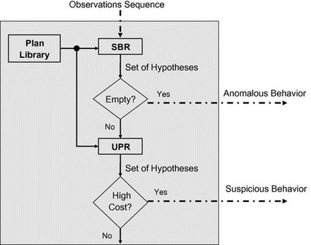
FIGURE 4.1 A hybrid adversarial plan-recognition system. Note: Inputs and outputs for the system shown with dashed arrows.

We begin by considering recognition of anomalous behavior using the symbolic plan-recognition algorithm (see Section 4.3.1). Here, the plan library represents normal behavior; any activity that does not match the plan library is considered abnormal. This approach can be effective in applications in which we have few or no examples of suspicious behavior (which the system is to detect) but many examples of normal behavior (which the system should ignore). This is the case, for instance, in many vision-based surveillance systems in public places.

A symbolic plan-recognition system is useful for recognizing abnormal patterns such as walking in the wrong direction, taking more than the usual amount of time to get to the security check, and so on. The symbolic recognizer can efficiently match activities to the plan library and rule out hypotheses that do not match. When the resulting set of matching hypotheses is empty, the sequence of observations is flagged as anomalous. The symbolic algorithm is very fast, since it rejects or passes hypotheses without ranking them.

However, detection of abnormal behavior is not sufficient. There are cases where a normal behavior should be treated as suspicious. In such cases, we cannot remove the behavior from the plan library (so as to make its detection possible using the anomalous behavior-detection scheme previously outlined), and yet we expect the system to detect it and flag it.

Section 4.4.2 presents the use of UPR for recognizing suspicious behavior. Here the plan library explicitly encodes behavior to be recognized, alongside any costs associated with the recognition of this behavior. This allows the UPR system to rank hypotheses based on their expected cost to the observing agent. As we shall see, this leads to being able to recognize potentially dangerous situations despite their low likelihood.

4.3.1 Efficient Symbolic Plan Recognition

We propose an anomalous behavior-recognition system; the input of the system is an observation sequence. The system is composed of a Symbolic Behavior Recognition module, which extracts coherent hypotheses from the observation sequence. If the set of hypotheses is empty, it declares the observation sequence as anomalous.

The symbolic plan-recognition algorithm, briefly described in the following, is useful for recognizing abnormal behavior, since it is very fast (no need to rank hypotheses) and can handle key capabilities required by modern surveillance applications. The reader is referred to Avrahami-Zilberbrand and Kaminka [3,4] for details.

The SBR’s plan library is a single-root directed graph, where vertices denote plan steps and edges can be of two types: decomposition edges decompose plan steps into substeps and sequential edges specify the temporal order of execution. The graph is acyclic along decomposition transitions.

Each plan has an associated set of conditions on observable features of the agent and its actions. When these conditions hold, the observations are said to match the plan. At any given time, the observed agent is assumed to be executing a plan decomposition path, root-to-leaf through decomposition edges. An observed agent is assumed to change its internal state in two ways. First, it may follow a sequential edge to the next plan step. Second, it may reactively interrupt plan execution at any time and select a new (first) plan. The recognizer operates as follows.

First, it matches observations to specific plan steps in the library according to the plan step’s conditions. Then, after matching plan steps are found, they are tagged by the timestamp of the observation. These tags are then propagated up the plan library so that complete plan paths (root-to-leaf) are tagged to indicate that they constitute hypotheses as to the internal state of the observed agent when the observations were made. The propagation process tags paths along decomposition edges. However, the propagation process is not a simple matter of following from child to parent. A plan may match the current observation yet be temporally inconsistent when a history of observations is considered. SBR is able to quickly determine the temporal consistency of a hypothesized recognized plan [3].

At the end of the SBR process, we are left with a set of current-state hypotheses (i.e., a set of paths through the hierarchy) that the observed agent may have executed at the time of the last observation.

The overall worst-case runtime complexity of this process is [3]. Here, is the number of plan steps that directly match the observations; is the maximum depth of the plan library. is typically very small, which is the number of specific actions that can match a particular observation.

The preceding presented the basics of the symbolic plan-recognition model. Extensions to this model, discussed in Avrahami-Zilberbrand [2] and Avrahami-Zilberbrand and Kaminka [4], address several challenges:

1. Reducing space complexity of matching complex multifeatured observations to the plan library

2. Dealing with plan execution duration constraints

3. Handling lossy observations, where an observation is intermittently lost

4. Handling interleaved plans where an agent interrupts a plan for another, only to return to the first later.

4.3.2 Efficient Utility-based Plan Recognition

This section presents an efficient hybrid technique used for recognizing suspicious behavior. Utility-based plan recognition allows the observer to incorporate a utility function into the plan-recognition process. With every potential hypothesis, we associate a utility to the observer should the hypothesis be correct. In adversarial UPR, this utility is the cost incurred by the observer. This allows choosing recognition hypotheses based on their expected cost to the observer, even if their likelihood is low.

The highly efficient symbolic plan recognizer introduced in Section 4.3.1 is used to filter hypotheses, maintaining only those that are consistent with the observations (but not ranking the hypotheses in any way). We then add an expected utility aggregation layer, which is run on top of the symbolic recognizer.

We briefly describe the basics of the UPR recognizer in this section. Avrahami-Zilberbrand [2] presents a general UPR framework, using influence diagrams as the basis for reasoning. Unfortunately, such reasoning is computationally expensive. Relying on a Markovian assumption, a less expressive but much more efficient UPR technique is used here. For its details, consult Avrahami-Zilberbrand [2] and Avrahami-Zilberbrand and Kaminka [5].

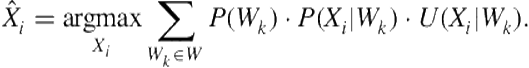
After getting all current-state hypotheses from the symbolic recognizer, the next step is to compute the expected utility of each hypothesis. This is done by multiplying the posterior probability of a hypothesis by its utility to the observer. We follow in the footsteps of—and then extend—the Hierarchical Hidden Markov Model [18] in representing probabilistic information in the plan library. We denote plan steps in the plan library by , where is the plan-step index and is its hierarchy depth, . For each plan step, there are three probabilities.

Sequential transition For each internal state , there is a state-transition probability matrix denoted by , where is the probability of making a sequential transition from the plan step to the plan step. Note that self-cycle transitions are also included in .

Interruption We denote by a transition to a special plan step , which signifies an interruption of the sequence of current plan step and immediate return of control to its parent, .

Decomposition transition When the observed agent first selects a decomposable plan step , it must choose between its (first) children for execution. The decomposition transition probability is denoted , the probability that plan step will initially activate plan step .

Observation probabilities Each leaf has an output emission probability vector . This is the probability of observing when the observed agent is in plan step . For presentation clarity, we treat observations as children of leaves and use the decomposition transition for the leaves as .

In addition to transition and interruption probabilities, we add utility information onto the edges in the plan library. The utilities on the edges represent the cost or gains to the observer, given that the observed agent selects the edge. For the remainder of the chapter, we use the term cost to refer to a positive value associated with an edge or node. As in the probabilistic reasoning process, for each node we have three kinds of utilities: (1) is the sequential-transition utility (cost) to the observer, conditioned on the observed agent transitioning to the next plan step, paralleling ; (2) is the interruption utility; and (3) is the decomposition utility to the observer, paralleling .

Figure 4.2 shows a portion of the plan library of an agent walking with or without a suitcase in the airport, occasionally putting it down and picking it up again; this example is discussed later. Note the end plan step at each level, and the transition from each plan step to this end plan step. This edge represents the probability to interrupt. The utilities are shown in diamonds (0 utilities omitted, for clarity). The transitions allowing an agent to leave a suitcase without picking it up are associated with large positive costs, since they signify danger to the observer.

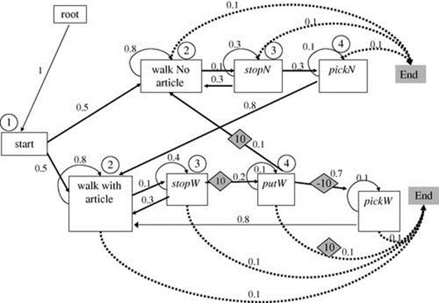
FIGURE 4.2 An example plan library. Note: Recognition timestamps (example in text) appear in circles. Costs appear in diamonds.

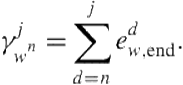
We use these probabilities and utilities to rank the hypotheses selected by the SBR. First, we determine all paths from each hypothesized leaf in timestamp to the leaf of each of the current-state hypotheses in timestamp . Then, we traverse these paths, multiplying the transition probabilities on edges by the transition utilities and accumulating the utilities along the paths. If there is more than one way to get from the leaf of the previous hypothesis to the leaf of the current hypothesis, then it should be accounted for in the accumulation. Finally, we can determine the most costly current plan step (the current-state hypothesis with maximum expected cost). Identically, we can also find the most likely current plan step for comparison.

Formally, let us denote hypotheses at time (each a path from root-to-leaf) as and the hypotheses at time as . To calculate the maximum expected-utility (most costly) hypothesis, we need to calculate for each current hypothesis its expected cost to the observer, , where is the sequence of observations thus far. Due to the use of SBR to filter hypotheses, we know that the observations in have resulted in hypothesis and that observation results in a new hypothesis . Therefore, under assumption of Markovian plan-step selection, .

The most costly hypothesis is computed in Eq. (4.1). We use , calculated in the previous timestamp, and multiply it by the probability and the cost to the observer of taking the step from to . This is done for all .

(4.1)

To calculate the expected utility , let be composed of plan steps and be composed of (the upper index denotes depth). There are two ways in which the observed agent could have gone from executing the leaf to executing the leaf . First, there may exist such that and have a common parent and is a direct decomposition of this common parent. Then, the expected utility is accumulated by climbing up vertices in (by takinginterrupt edges) until we hit the common parent and then climbing down (by taking first child decomposition edges) to . Or, in the second case, is reached by following a sequential edge from a vertex to a vertex .

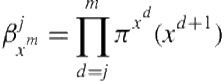
In both cases, the probability of climbing up from a leaf at depth to a parent , where , is given by

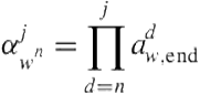(4.2)

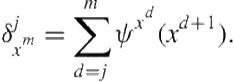
and the utility is given by

(4.3)

The probability of climbing down from a parent to a leaf is given by

(4.4)

and the utility is given by

(4.5)

Note that we omitted the plan-step index and left only the depth index for presentation clarity.

Using , and , and summing over all possible ’s, we can calculate the expected utility (Eq. (4.6)) for the two cases in which a move from to is possible:

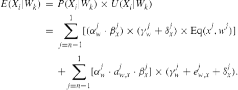(4.6)

The first term covers the first case (transition via interruption to a common parent). Let return if and otherwise. The summation over accumulates the probability, multiplying the utility of all ways of interrupting a plan , climbing up from to the common parent , and following decompositions down to .

The second term covers the second case, where a sequential transition is taken. is the probability of taking a sequential edge from to , given that such an edge exists () and that the observed agent is done in . To calculate the expected utility, we first multiply the probability of climbing up to a plan step that has a sequential transition to a parent of , then we multiply in the probability of taking the transition; after that we multiply in the probability of climbing down again to . Then, we multiply in the utility summation along this path.

A naive algorithm for computing the expected costs of hypotheses at time can be expensive to run. It would go over all leaves of the paths in and for each traverse the plan library until getting to all leaves of the paths we got in timestamp . The worst-case complexity of this process is , where is the plan library size and is the number of observations.

In Avrahami-Zilberbrand [2] we presented a set of efficient algorithms that calculate the expected utilities of hypotheses (Eq. (4.1)) in worst-case runtime complexity , where is the depth of the plan library ( are as before). The reader is referred to Avrahami-Zilberbrand [2] for details.

4.4 Experiments to Detect Anomalous and Suspicious Behavior

This section evaluates the system that was described in Section 4.3 in realistic problems of recognizing both types of adversarial plans: anomalous and suspicious behaviors. We discuss recognition of anomalous behavior in Section 4.4.1. In Section 4.4.2, we turn to the use of UPR for recognizing suspicious behavior.

4.4.1 Detecting Anomalous Behavior

We evaluate the use of SBR for anomalous behavior recognition using real-world data from machine vision trackers, which track movements of people and report on their coordinate positions. We conduct our experiments in the context of a vision-based surveillance application. The plan library contains discretized trajectories that correspond to trajectories known to be valid. We use a specialized learning algorithm, described briefly in The learning algorithm subsection, to construct this plan library.

The Evaluation using CAVIAR data subsection describes in detail the experiments we conducted, along with their results on video clips and data from the CAVIAR project [13]. The AVNET consortium data subsection presents results from datasets gathered as part of our participation in a commercial R&D consortium (AVNET), which developed technologies for detection of criminal, or otherwise suspicious, objects and suspects.

To evaluate the results of the SBR algorithms, we distinguish between two classes of observed trajectories: anomalous and nonanomalous. The true positives are the anomalous trajectories that were classified correctly. True negatives are, similarly, nonanomalous trajectories that were classified correctly. The false positives are the nonanomalous trajectories that were mistakenly classified as anomalous. The false negatives are the number of anomalous trajectories that were not classified as anomalous.

We use the precision and recall measures that are widely used in statistical classification. A perfect precision score of 1 means that every anomalous trajectory that was labeled as such was indeed anomalous (but this says nothing about anomalous trajectories that were classified as nonanomalous). A perfect recall score of 1 means that all anomalous trajectories were found (but says nothing about how many nonanomalous trajectories were also classified as anomalous). The reader is referred to [58] for a detailed description.

4.4.1.1 The learning algorithm

We use a simple learning algorithm that was developed for the purpose of building plan-recognition libraries based on examples of positive (valid) trajectories only. The learning algorithm is fully described in Avrahami-Zilberbrand [2] and Kaminka et al. [31,32]. We provide a description of its inputs and outputs next, as those are of interest here.

The learning algorithm receives a training set that contains observation sequences, . Each observation sequence is one trajectory of an individual target composed of all observations (samples) , where is an ordering index within . Each observation is a tuple , where are Cartesian coordinates of points within and is a time index.

The learning algorithm divides the work area W using a regular square-based grid. Each observation is assigned a square that contains this point. For each trajectory of an individual target () in the training set, it creates a sequence of squares that represents that trajectory.

The output of the algorithm is a set of discretized trajectories, each a sequence of grid cells that are used together as the plan library for the recognition algorithm. Figure 4.3 shows a work area that is divided into nine squares with one trajectory. The output of the algorithm is the sequence of squares that defines that trajectory (at right of figure).

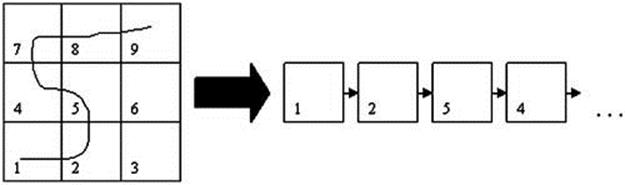
FIGURE 4.3 Result of running naive learning algorithm on one trajectory.

The grid’s square cell size is an input for the learning algorithm. By adjusting the size of the square, we can influence the relaxation of the model. By decreasing the size of the square, the learned library is more strict (i.e., there is less generalization); in contrast, too large a value would cause overgeneralization. Small square size may result in overfitting; a trajectory that is very similar to an already-seen trajectory but differs slightly will not fit the model. By increasing the size of the square, the model is more general and is less sensitive to noise, but trajectories that are not similar might fit.

People are rarely in the exact same position twice. As a result, the training set may contain many sample trajectories that differ by very small distances. Part of the challenge in addressing this lies in adjusting the square size, as described previously. However, often a part of a trajectory would fall just outside the cell that contains the other examples of the same trajectories.

To solve this, the learning algorithm has another input parameter called position overlap size. Position overlap prevents overfitting to the training data by expanding each square such that it overlaps with those around it (see Figure 4.4, where the position overlap is shown for square 5). Any point in a trajectory that lies in an overlapping area is defined to match both the overlapping square and the square within which it falls. Thus, for instance, a point within cell 3 in Figure 4.4 (i.e., top right corner within the darkened overlapping area of cell 5) would match cell 3 and 5, as well as 6 and 2 (since these cells also have their own overlapping areas). Essentially, this is analogous to having nonzero observation-emitting probabilities for the same observation from different states in a Hidden Markov Model.

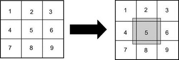
FIGURE 4.4 Demonstrating position overlap. Note: This shows the additional position overlap for square number 5.

4.4.1.2 Evaluation using CAVIAR data

We use two sets of real-world data to evaluate SBR’s performance as an anomalous behavior recognizer. Experiments with the first set are described in this section. The second set is described in the next subsection.

The first set of experiments were conducted on video clips and data from the CAVIAR [13] project.² The CAVIAR project contains a number of video clips with different scenarios of interest: people walking alone, standing in one place and browsing, and so on. The videos are pixels, 25 frames per second. Figure 4.5 shows a typical frame. Originally, the CAVIAR data were gathered to allow comparative evaluations of machine-vision tracking systems. To do this, the maintainers of the CAVIAR dataset determined the ground truth positions of subjects, in pixel coordinates, by hand labeling the images.

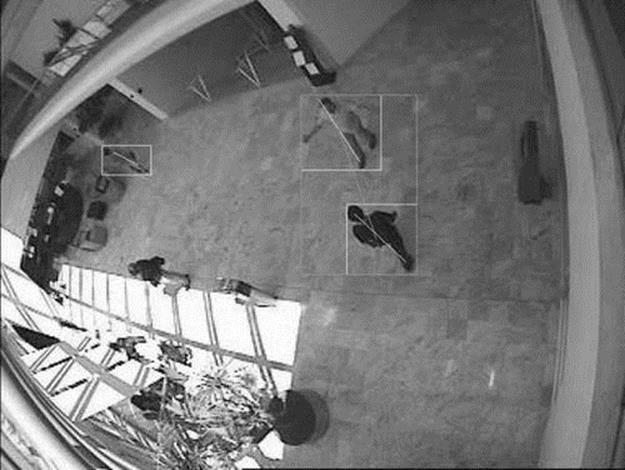
FIGURE 4.5 A typical frame of image sequence in the CAVIAR project.

We use the ground-truth data to simulate the output of realistic trackers at different levels of accuracy. To do this, each ground-truth position of a subject, in pixel coordinates, is converted by homography (a geometric transformation commonly used in machine vision) to a position in the 2D plane on which the subjects move (in centimeters). Then we add noise with normal distributions to simulate tracking errors. Higher variance simulates less accurate trackers, and low variance simulates more accurate trackers. In the experiments reported on in the following, we use a standard deviation of 11 cm diagonal (8 cm vertical and horizontal). The choice of noise model and parameters is based on information about state-of-the-art trackers (e.g., see McCall and Trivedi [46]).

To create a large set of data for the experiments, representing different tracking instances (i.e., the tracking results from many different video clips), we simulated multiple trajectories of different scenarios and trained the learning system on them to construct a plan library. This plan library was then used with different trajectories to test the ability of the algorithms to detect abnormal behavior.

In the first experiment, we tested simple abnormal behavior. We simulated three kinds of trajectories:

1. Curved path A. Taken from the first set in CAVIAR, titled One person walking straight line and return. In this video, a subject is shown walking along a path and then turning back. We took the first part, up to the turn back, as the basis for normal behavior in this trajectory.

2. U-turn. As in 1. but then including the movement back.

3. Curved path B. Taken from the CAVIAR set, titled One person walking straight, which is similar to 1. but curves differently toward the end. We use this to evaluate the system’s ability to detect abnormal behavior (e.g., as compared to Curved path A).

Figure 4.6 shows the three trajectories. The arrow shows the starting position of the trajectories. The endpoints lie at the other end (movement right to left).

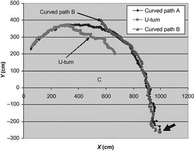
FIGURE 4.6 Three trajectories. Legal path (curved path A), suspicious path (curved path B), and return path (U-turn) from CAVIAR data. The thick arrow points at the starting point.

We created 100 simulated trajectories of each type, for a total of 300 trajectories. We trained a model on 100 noisy trajectories from Curved path A, using the learning system described in The learning algorithm section. In this experiment, we fixed the grid cell size to 55 cm, and we vary the plan library relaxation parameter (called position overlap size). The cell size was chosen such that it covered the largest distance between two consecutive points in the training set trajectories.

Figure 4.7 shows the true positives versus false positives. The X-axis is the plan library relaxation, and the Y-axis is the number of trajectories (subjects). We can see that the system starts stabilizing in a plan library relaxation of 11 (number of false positives is 0), and after a plan library relaxation of 15, the system is too relaxed; the number of abnormal trajectories not detected slowly increases.

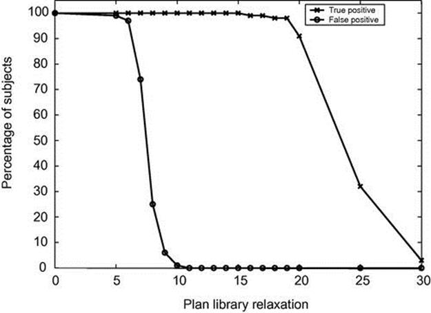
FIGURE 4.7 True positives versus false positives on CAVIAR data.

Figure 4.8 shows the precision and recall of the system. The X-axis is the plan library relaxation, and the Y-axis is the number of trajectories (subjects). The precision increases until a perfect score of 1 from relaxation 11. The recall starts with a perfect score of 1 and decreases slowly from relaxation 16. As in Figure 4.7, for values of plan library relaxation of 11 through 15, we get a perfect precision and a perfect recall of 1. Despite the optimistic picture that these results portray, it is important to remember that the results ignore the time for detection. However, in practice, the time for detection matters.

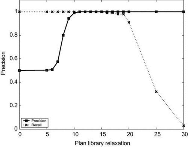
FIGURE 4.8 Precision and recall on CAVIAR data.

Figure 4.9 shows the time for detecting the abnormal behavior with standard deviation bars. The X-axis measures the plan library relaxation parameter range, and the Y-axis measures the time (in seconds) before passes until the detection of abnormal behavior. In this figure, we can see that before a relaxation of 12 cm, the time for detection is negative; this is because we detect too early (i.e., before the abnormal behavior takes place). Two seconds is the maximum of the graph, since this is the time when the scene was over; therefore detecting at 2 s is too late.

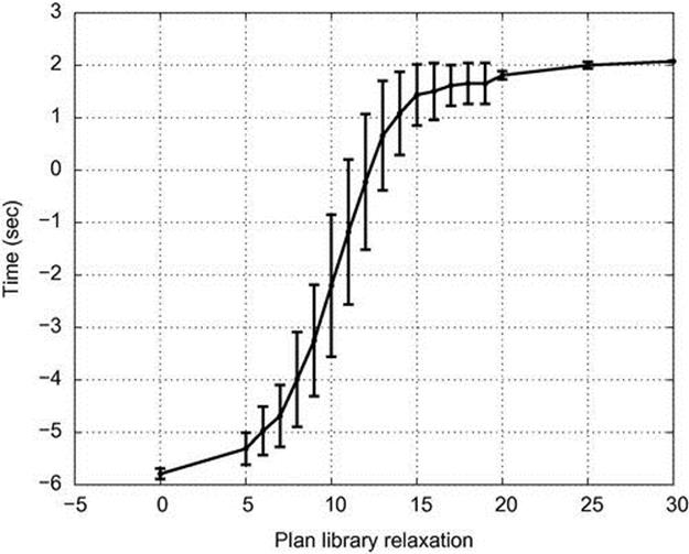
FIGURE 4.9 Time for detection of a suspicious path on CAVIAR data.

Figure 4.10 shows the trade-off between detecting too late and detecting too early as a function of plan library relaxation, where too early is before the split and too late is the end of the abnormal path. The X-axis is the plan library relaxation, and the Y-axis is the percentage of subjects detected too early or too late. We can see that a relaxation of 16 gives the best results of too early and too late. After a relaxation of 16, the percentage of trajectories that we detect too late slowly increases.

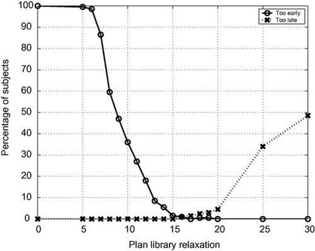
FIGURE 4.10 Too early detection and too late detection on CAVIAR data.

The recognition algorithm also is capable of detecting anomalous behavior in direction, not only in position. The following experiment demonstrates this capability; here, we evaluate the use of the system in identifying the U-turn trajectories in the dataset. We sampled 100 instances of the U-turn trajectory with Gaussian noise and checked the time for detection. We trained a model on the same 100 noisy trajectories from curved path A that we used in the first experiment.

We first examine the time to detect a U-turn as an abnormal behavior. Figure 4.11 shows the time for detecting abnormal behavior versus the plan library relaxation. The X-axis is the plan library relaxation, and the Y-axis is the time (sec) passed until detecting the U-turn. We can see that until plan library relaxation of about 10, the time for detection is negative, since we detect too early (i.e., before the U-turn behavior takes place), and the standard deviation is high. The maximum detection time is 2.5 s after the turn takes place. Figure 4.12 demonstrates the position on the trajectory 1 s after the turn, 2 s after the turn, and 10 s after the turn.

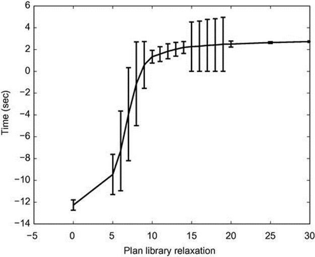
FIGURE 4.11 Time for detecting U-turn on CAVIAR data.

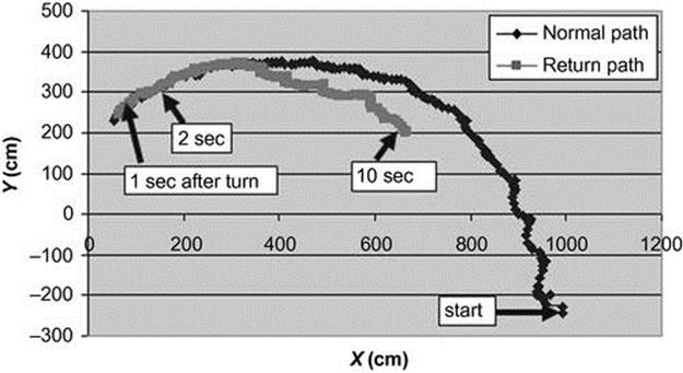
FIGURE 4.12 U-turn on CAVIAR data.

Figure 4.13 shows the precision and recall for the U-turn experiment as a function of the time. The plan library relaxation was set to 15, which is the best relaxation according to the first experiment. The precision has the perfect score of 1 for a plan relaxation of 15 (every suspect labeled as a suspect was indeed a suspect). The recall starts from score 0 and gradually increases, and after about 2.5 s it gets the perfect score of 1 (all suspects were found 2.5 s after the turn).

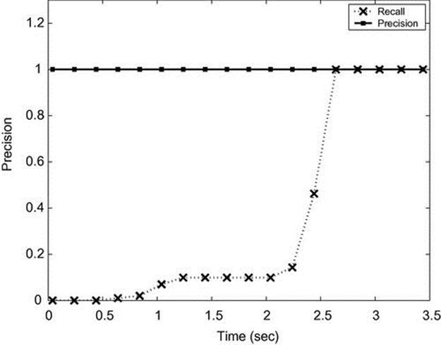
FIGURE 4.13 Precision and recall for U-turn versus time on CAVIAR data.

4.4.1.3 AVNET consortium data

Parts of our work were funded through the AVNET consortium, a government-funded project that includes multiple industrial and academic partners, for development of suspicious activity-detection capabilities. As part of this project, we were given the tracking results from a commercial vision-based tracker developed by consortium partners.

We used the consortium’s datasets to evaluate our algorithm. In the first experiment, we got 164 trajectories, all with normal behavior. We ran a 10-fold cross-validation test on the dataset to test performance. We divided the 10 datasets so that each contained 148 trajectories for training and 16 trajectories for test (except the last test that contained 20 trajectories for test and 144 for training). We learned a model with its square size fixed to be the size of the maximum step in the data (31), and the position overlap to be 10.

We checked the number of false positives (the number of nonsuspects that were mistakenly classified as suspects). Table 4.1 shows the results. We can see that the maximum number of false positives is 1 out of 16 (). On average, across the trials, the percentage of the false positives is .

Table 4.1

Percentage of False Positives in AVNET Data

The next two experiments evaluate the recognition of anomalous behavior using the AVNET dataset. In the first experiment, we were given data that consisted of 18 trajectories (432 single points). We learned from this data a model, with a grid size of 31 and a position overlap of 10, as in the first experiment. We tested it against a single trajectory with a U-turn pattern. Figure 4.14 shows all of the 18 trajectories; the turn pattern, which was found suspicious, is marked in bold by the recognition system. The arrows point to the start position and the turn position.

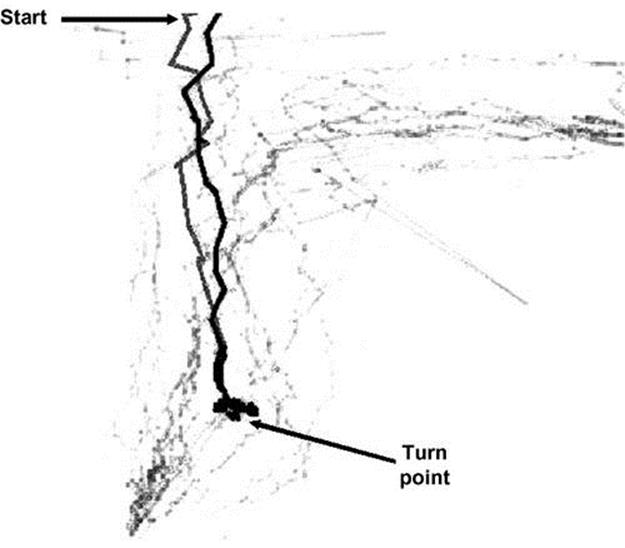
FIGURE 4.14 Detecting U-turn on AVNET data.

In the second experiment of evaluating anomalous behavior, we show that detecting abnormal behavior based on spatial motion is not enough. There is also a need to recognize abnormal behavior in time. For instance, we would like to recognize as abnormal someone who stays in one place an excessive amount of time or who moves too slowly or too quickly.

We were given a dataset consisting of 151 trajectories (a total of 4908 single points). In this experiment, we learned on this data a model, with grid size of 31 and position overlap of 10, as in the first experiment. We tested it against a single trajectory of standing in place for a long duration. Figure 4.15shows all of the 151 trajectories. The trajectory that was detected as anomalous by the recognition system is shown in bold. The arrows point at the start position and the standing position.

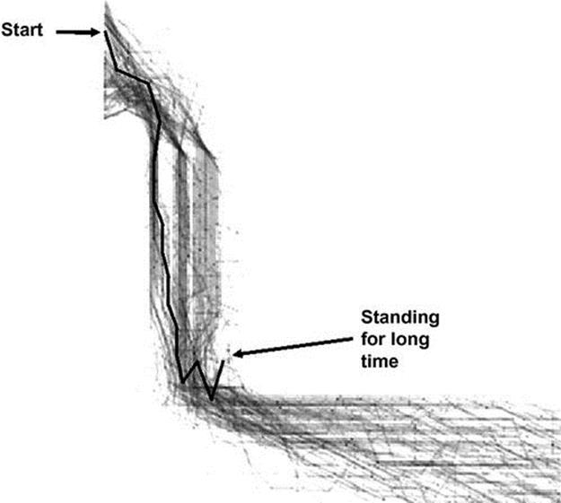
FIGURE 4.15 Detecting standing for long time on AVNET data.

4.4.2 Detecting Suspicious Behavior

To demonstrate the capabilities of UPR, and its efficient implementation as described in Section 4.3, we tested the capabilities of our system in three different recognition tasks. The domain for the first task consisted of recognizing passengers who leave articles unattended, as in the previous example. In the second task, we show how our algorithms can catch a dangerous driver who cuts between two lanes repeatedly. The last experiment’s intent is to show how previous work, which has used costs heuristically [56], can now be recast in a principled manner. All of these examples show that we should not ignore observer biases, since the most probable hypothesis sometimes masks hypotheses that are important for the observer.

4.4.2.1 Leaving unattended articles

It is important to track a person who leaves her articles unattended in the airport. It is difficult, if not impossible, to catch this behavior using only probabilistically ranked hypotheses. We examine the instantaneous recognition of costly hypotheses.

We demonstrate the process using the plan library shown earlier in Figure 4.2. This plan library is used to track simulated passengers in an airport who walk about carrying articles, which they may put down and pick up again. The recognizer’s task is to detect passengers who put something down and then continue to walk without it. Note that the task is difficult because the plan steps are hidden (e.g., we see a passenger bending but cannot decide whether she picks something up, puts something down, or neither); we cannot decide whether a person has an article when walking away.

For the purposes of a short example, suppose that in time (see Figure 4.2), the SBR had returned that the two plan steps marked walk match the observations (walkN means walking with no article, walkW signifies walking with an article), in time the two plan steps match ( and ), and in time the plan steps and match (e.g., we saw that the observed agent was bending).

The probability in will be (the probability of in previous timestamp is 0.5, then following sequential link to ), and in the same way . Normalizing the probabilities for the current time and . The expected utility in time is . The expected utility of is 0. The expected costs, rather than likelihoods, raise suspicions of a passenger putting down an article (perhaps not picking it up).

Let us examine a more detailed example. We generated the following observations based on the plan library shown in Figure 4.2: Suppose that in timestamps the passenger walks in an airport, but we cannot tell whether she has a dangerous article in her possession. In timestamps she stops, then at time we see her bending but cannot tell whether it is to put down or to pick up something. In timestamps , she walks again.

Figure 4.16 shows the results from the recognition process for these observations. The X-axis measures the sequence of observations in time. The probability of different leaves (corresponding to hypotheses) is shown on the Y-axis in the upper graph; expected costs are shown in the lower graph. In both, the top-ranking hypothesis (after each observation) is the one with a value on the Y-axis that is maximal for the observation.

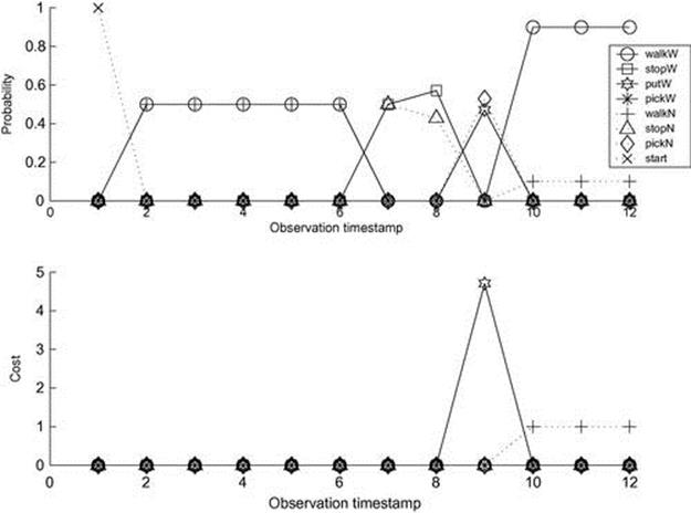
FIGURE 4.16 Leaving unattended articles: probabilities and costs.

In the probabilistic version (upper graph), we can see that the probabilities, in time , are 0.5 since we have two possible hypotheses of walking, with or without an article ( and ). Later when the person stops, there are again two hypotheses, and . Then, in two plan steps match the observations: and , where the prior probability of is greater than (after all, most passengers do not leave items unattended). As a result, the most likely hypothesis for the remainder of the sequence is that the passenger is currently walking with her article in hand, walkW.

In the lower graph we can see a plot of the hypotheses, ranked by expected cost. At time when the agent picks or puts something, the cost is high (equal to 5); then in timestamp , the top-ranking hypothesis is walkN, signifying that the passenger might have left an article unattended. Note that the prior probabilities on the behavior of the passenger have not changed. What is different here is the importance (cost) we attribute to observed actions.

4.4.2.2 Catching a dangerous driver

Some behavior becomes increasingly costly, or increasingly gainful, if repeated. For example, a driver switching a lane once or twice is not necessarily acting suspiciously. But a driver zigzagging across two lanes is dangerous. We demonstrate here the ability to accumulate costs of the most costly hypotheses in order to capture behavior with expected costs that are prohibitive over time.

Figure 4.17 shows two lanes, left and right, in a continuous area divided by a grid. There are two straight trajectories and one zigzag trajectory from left to right lane. From each position, the driver can begin moving to the next cell in the row (straight) or to one of the diagonal cells. We emphasize that the area and movements are continuous—the grid is only used to create a discrete state space for the plan library. Moreover, the state space is hidden: A car in the left lane may be mistakenly observed (with small probability) to be in the right lane, and vice versa.

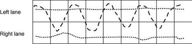
FIGURE 4.17 Simulated trajectories for drivers.

Each grid cell is a plan step in the plan library. The associated probabilities and utilities are as follows: The probability for remaining in a plan step (for all nodes) is 0.4. The probability of continuing in the same lane is 0.4. The probability of moving to either diagonal is 0.2. All costs are 0, except when moving diagonally, where the cost is 10. Observations are uncertain; with 0.1 probability, an observation would incorrectly report on the driver being in a given lane.

We generated 100 observation sequences (each of 20 observations) of a driver zigzagging and 100 sequences of a safe driver. The observations were sampled (with noise) from the trajectories (i.e., with observation uncertainty). For each sequence of observations, we accumulated the cost of the most costly hypothesis, along the 20 observations. We now have 100 samples of the accumulated costs for a dangerous driver and 100 samples of the costs for a safe driver. Depending on a chosen threshold value, a safe driver may be declared dangerous (if its accumulated cost is greater than the threshold) and a dangerous driver might be declared safe (if its accumulated cost is smaller than the threshold).

Figure 4.18 shows the confusion error rate as a function of the threshold. The error rate measures the percentage of cases (out of 100) incorrectly identified. The figure shows that a trade-off exists in setting the threshold in order to improve accuracy. Choosing a cost threshold at 50 results in high accuracy in this particular case: All dangerous drivers will be identified as dangerous, and yet 99% of safe drivers will be correctly identified as safe.

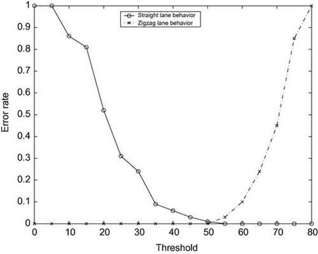
FIGURE 4.18 Confusion error rates for different thresholds for dangerous and safe drivers.

4.4.2.3 Air-combat environment

Tambe and Rosenbloom [56] used an example of agents in a simulated air-combat environment to demonstrate the RESC plan-recognition algorithm. RESC heuristically prefers a single worst-case hypothesis, since an opponent is likely to engage in the most harmful maneuver in an hostile environment. The authors [56] showed this heuristic in action in simulated air combat, where the turning actions of the opponent could be interpreted as either leading to it running away or to its shooting a missile.

RESC prefers the hypothesis that the opponent is shooting. However, unlike UPR, RESC will always prefer this hypothesis, regardless of its likelihood, and this has proved problematic [56]. Moreover, given several worst-case hypotheses, RESC will arbitrarily choose a single hypothesis to commit to, again regardless of its likelihood. Additional heuristics were therefore devised to control RESC’s worst-case strategy [56].

We generalize this example to show UPR subsumes RESC’s heuristic in a principled manner. For shooting a missile (which has infinite cost) versus running away, we consider hypotheses of invading airspace versus runaway, where invading the observer’s airspace is costly but not fatal. Figure 4.19 shows models of two types of opponents: an aggressive one (left subfigure) who is more likely to shoot (0.8 a priori probability) than to run away (0.2), and a cowardly opponent (right subfigure) who is more likely to run away.

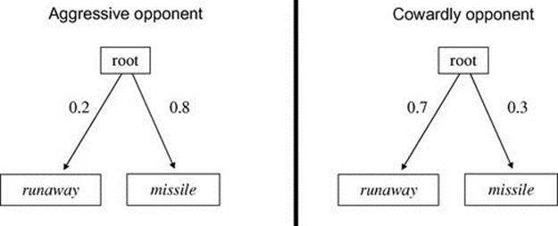
FIGURE 4.19 Air-combat environment: two types of opponents.

Note that these models are structurally the same; the assigned probabilities reflect the a priori preferences of the different opponent types. Thus, an observation matching both hypotheses will simply lead to both of them being possible, with different likelihoods. The maximum posterior hypothesis in the aggressive case will be that the opponent is trying to invade our airspace. In the cowardly case, it would be that the opponent is running away. RESC’s heuristic would lead it to always select the aggressive case, regardless of the likelihood.

In contrast, UPR incorporates the biases of an observing pilot much more cleanly. Because it takes the likelihood of hypotheses into account in computing the expected cost, it can ignore sufficiently improbable (but still possible) worst-case hypotheses in a principled manner. Moreover, UPR also allows modeling optimistic observers, who prefer best-case hypotheses.

Table 4.2 presents three cost models. In the first case, the runaway plan step will get 0 cost and invade a high cost (10). This is an observer who is worried that his airspace is being invaded but not gaining anything from scaring the opponent away. In the second case, the runaway plan step will get negative cost (i.e., a gain for the observer). In the third case, the costs are the same. Tables 4.3 and 4.4 show the recognition results. The first row In Tables 4.3 and 4.4 shows the results of following only the probabilistic reasoning in each model. The next three rows show the hypothesis costs for each hypothesis in each of the three cases in Table 4.2.

Table 4.2

Three Cases of Utilities for Figure 4.19

Table 4.3

Aggressive Opponent: Result Utilities for Figure 4.19

Table 4.4

Cowardly Opponent: Result Utilities for Figure 4.19

In the cases of the aggressive opponent, the most costly, or the most probable hypothesis, is the invade hypothesis. However, in the cowardly opponent case, the answer depends on the utility model. In cases A and B, where we gave a high cost for missile, the most probable hypothesis stays runaway but the costly hypothesis is missile. In the third case, C, since we gave neutral costs (same for the two plan steps), we got a result that is the same as in the probability model, meaning runaway. The conclusion is that the probabilistic model is not enough in case we want to incorporate biases of the observer, in this case that the missile plan step is harmful for the observer.

This generalization of the original example in Tambe and Rosenbloom [56] demonstrates that the heuristic worst-case preference of RESC is subsumed by the principled use of decision theoretic reasoning in our algorithms. In addition, the complexity analysis in earlier sections shows that such reasoning does not necessarily entail significant computational costs. RESC’s runtime complexity is linear in the size of plan library; UPR’s is polynomial.

4.5 Future Directions and Final Remarks

In this chapter, we concentrated on efficient hybrid adversarial plan-recognition algorithms (Section 4.3) and their contribution to the domain of detecting anomalous and suspicious behavior (Section 4.4). The two main contributions of this chapter are as follows:

• First, we presented an anomalous behavior recognition model using the Symbolic Behavior Recognizer (SBR) that is capable of answering the plan library membership query very efficiently [3,4]. Here, the plan library represents normal behavior; any activity that does not match the plan library is flagged as anomalous. We demonstrated its use in two sets of experiments with trajectories created by machine-vision systems.

• Second, we presented a suspicious behavior-recognition model using utility-based plan recognition (UPR) [2,5]. This is a general model of plan recognition that allows the observer to incorporate her own biases and preferences—in the form of a utility function—into the plan-recognition process. Here, the plan library explicitly represents suspicious behavior; any activity that matches the model will be assumed to be suspicious. We demonstrate the capabilities of the suspicious behavior-recognition model in three different domains and also its principled generalization of previous (heuristic) adversarial plan-recognition work [56].

The hybrid system presented is an instantiation of a more general approach to keyhole adversarial plan recognition, combining two approaches: one detecting anomalous behavior and the other detecting suspicious behavior. This approach leaves open many challenges, including:

• Formally defining multiagent plan recognition (MAPR) queries in adversarial settings, and exploring methods for anomalous and suspicious plan recognition in multiagent settings.

• Following up on Kaluža et al.[53], continuing to explore methods for UPR for suspicious plan recognition, which maintain computational tractability but with greater expressiveness.

• Most plan-recognition literature—and this chapter is no different—ignores intended recognition, where the adversary knows it is being observed and acts accordingly (for a recent exception see Lisy et al. [39]). In adversarial settings, assuming that the adversary knows it is being observed can cause a computational blow-up; this is because even when an another agent appears to not be suspicious, the system must necessarily assume it is only acting as such because it is being observed. Thus, pruning hypotheses is necessarily difficult.

References

1. Adams JA. Human management of a hierarchical system for the control of multiple mobile robots. PhD thesis, University of Pennsylvania; 1995.

2. Avrahami-Zilberbrand D. Efficient hybrid algorithms for plan recognition and detection of suspicious and anomalous behavior. PhD thesis, Bar Ilan University; 2009.

3. Avrahami-Zilberbrand D, Kaminka GA. Fast and complete symbolic plan recognition. Proceedings of the International Joint Conference on Artificial Intelligence. 2005:653-658.

4. Avrahami-Zilberbrand D, Kaminka GA. Fast and complete symbolic plan recognition. IJCAI Workshop on Modeling Other Agents from Observations. 2005.

5. Avrahami-Zilberbrand D, Kaminka GA. Incorporating observer biases in keyhole plan recognition (efficiently!). Proceedings of 22nd National Conference on Artificial Intelligence. 2007:944-949.

6. Baker C, Tenenbaum J. Modeling human plan recognition using Bayesian theory of mind. In: Sukthankar G, Goldman RP, Geib C, Pynadath DV, Bui HH, eds. Plan, activity, and intent recognition. Waltham, MA: Morgan Kaufmann Publishers; 2014:177-206.

7. Blaylock N, Allen J. Fast hierarchical goal schema recognition. Proceedings of the 21st National Conference on Artificial Intelligence. 2006:796-801.

8. Boyen X, Koller D. Tractable inference for complex stochastic processes. Proceedings of the 14th Annual Conference on Uncertainty in AI. 1998:33-42.

9. Brand M, Oliver N, Pentland A. Coupled hidden Markov models for complex action recognition. Proceedings of the 1997 Conference on Computer Vision and Pattern Recognition. 1997:994.

10. Bui H. A general model for online probabilistic plan recognition. Proceedings of the International Joint Conference on Artificial Intelligence. 2003.

11. Bui H, Venkatesh S, West G. Policy recognition in the abstract hidden Markov models. J Art Intell Res. 2002;17:451-499.

12. Bui HH, Phung D, Venkatesh S, Phan H. The hidden permutation model and location-based activity recognition. Proceedings of 23rd National Conference on Artificial Intelligence. 2008.

13. EC-funded CAVIAR project/IST 2001-37540, available at: <http://homepages.inf.ed.ac.uk/rbf/CAVIAR/>.

14. Cooper GF. The computational complexity of probabilistic inference using Bayesian belief networks (research note). Art Intell. 1990;42(2–3):393-405.

15. Cupillard F, Avanzi Alberto, Bremond F, Thonnat M. Video understanding for Metro surveillance. Proceedings of the IEEE ICNSC 2004 Special Session on Intelligent Transportation Systems. 2004:186-1891.

16. Doyle RJ. Determining the loci of anomalies using minimal causal models. Proceedings of the International Joint Conference on Artificial Intelligence. 1995:1821-1827.

17. Duong TV, Bui HH, Phung DQ, Venkatesh S. Activity recognition and abnormality detection with the switching hidden semi-Markov models. IEEE International Conference on Computer Vision and Pattern Recognition. 2005:838-845.

18. Fine S, Singer Y, Tishby N. The hierarchical hidden Markov model: analysis and applications. Mach Learn. 1998;32(1):41-62.

19. Geib C. Delaying commitment in plan recognition using combinatory categorial grammars. International Joint Conference on Artificial Intelligence. 2009:1702-1707.

20. Geib C, Goldman R. Recognizing plans with loops represented in a lexicalized grammar. Proceedings of the 25th AAAI Conference on Artificial Intelligence. 2011:958-963.

21. Geib C, Steedman M. On natural language processing and plan recognition. International Joint Conference on Artificial Intelligence. 2007:1612-1617.

22. Geib CW. Assessing the complexity of plan recognition. Proceedings of the 19th National Conference on Artificial Intelligence. 2004:507-512.

23. Geib CW, Goldman RP. Plan recognition in intrusion detection systems. DARPA Information Survivability Conference and Exposition. 2001:329-342.

24. Geib CW, Harp SA. Empirical analysis of a probabilistic task tracking algorithm. AAMAS Workshop on Modeling Other Agents from Observations. 2004.

25. Ghahramani Z, Jordan MI. Factorial hidden Markov models. In: Touretzky DS, Mozer MC, Hasselmo ME, eds. Proceedings of the Conference Advances in Neural Information Processing Systems. 1995:472-478.

26. Hilary B, Shaogang G. Advanced visual surveillance using Bayesian networks. International Conference on Computer Vision. 1995:111-123.

27. Hongeng S, Brémond F, Nevatia R. Bayesian framework for video surveillance application. Proceedings of the 15th International Conference on Pattern Recognition. 2000:164-170.

28. Hu DH, Yang Q. CIGAR: concurrent and interleaving goal and activity recognition. Proceedings of 23rd National Conference on Artificial Intelligence. 2008:1363-1368.

29. Jarvis P, Lunt T, Myers K. Identifying terrorist activity with AI plan recognition technology. Proceedings of the Sixth Innovative Applications of Artificial Intelligence Conference. 2004:858-863.

30. Kaminka GA. Detecting disagreements in large-scale multi-agent teams. J Autonom Agents Mul-Agent Sys. 2009;18(3):501-525.

31. Kaminka GA, Merdler E, Avrahami D. Advanced unsupervised spatial learning algorithm for the AVNET37 consortium: final report (in hebrew). Technical Report MAVERICK 2006/01, Bar Ilan University, Computer Science Department, MAVERICK Group; 2006.

32. Kaminka GA, Merdler E, Avrahami D. Advanced unsupervised spatial learning algorithm for the AVNET37 consortium: interim report (in Hebrew). Technical Report MAVERICK 2006/01, Bar Ilan University, Computer Science Department, MAVERICK Group; 2006.

33. Kaminka GA, Pynadath DV, Tambe M. Monitoring teams by overhearing: a multi-agent plan recognition approach. J Art Intell Res. 2002;17:83-135.

34. Kaminka GA, Tambe M. Robust multi-agent teams via socially-attentive monitoring. J Art Intell Res. 2000;12:105-147.

35. Khalastchi E, Kalech M, Kaminka GA, Lin R. Online anomaly detection in unmanned vehicles. Proceedings of the 10th International Joint Conference on Autonomous Agents and Multi-Agent Systems. 2011:115-122.

36. Kjærulff U. A computational scheme for reasoning in dynamic probabilistic networks. Proceedings of the Conference on Uncertainty in Artificial Intelligence. 1992:121-129.

37. Lane T, Brodley CE. Temporal sequence learning and data reduction for anomaly detection. ACM Trans Inform Sys Sec. 1999;2(3):295-331.

38. Liao L, Fox D, Kautz HA. Learning and inferring transportation routines. Proceedings of the 19th National Conference on Artificial Intelligence. 2004:348-353.

39. Lisy V, Pibil R, Stiborek J, Bosansky B, Pechoucek M. Game-theoretic approach to adversarial plan recognition. In: de Raedt L, Bessiere C, Dubois D, Doherty P, Frasconi P, Heintz F, eds. 20th European Conference on Artificial Intelligence. Frontiers in artificial intelligence and applications. vol. 242. IOS Press; 2012:546-551.

40. Mahajan D, Kwatra N, Jain S, Kalra P, Banerjee S. A framework for activity recognition and detection of unusual activities. ICVGIP. 2004:15-21.

41. Mao W, Gratch J. Decision-theoretic approaches to plan recognition. In USC/ICT Technical Report; 2004.

42. Mao W, Gratch J. A utility-based approach to intention recognition. Proceedings of the AAMAS Workshop on Modeling Other Agents from Observations. 2004.

43. Marhasev E, Hadad M, Kaminka GA, Feintuch U. The use of hidden semi-Markov models in clinical diagnosis maze tasks. Intell Data Anal. 2009;13(6):943-967.

44. Nguyen N, Phung D, Venkatesh S, Bui H. Learning and detecting activities from movement trajectories using the hierarchical hidden Markov model. IEEE International Conference on Computer Vision and Pattern Recognition. 2005:955-960.

45. Niu W, Long J, Han D, Wang Y-F. Human activity detection and recognition for video surveillance. Proceedings of the IEEE Multimedia and Expo Conference. 2004:719-722.

46. McCall Joel C, Trivedi Mohan M. Performance evaluation of a vision based lane tracker designed for driver assistance systems. IEEE intellient vehicles symposium. 2005:153-158.

47. Oliver N, Horvitz E, Garg A. Layered representations for human activity recognition. Proceedings of the Fourth IEEE International Conference on Multimodal Interfaces. 2002:831-843.

48. Pynadath DV, Marsella S. Psychsim: modeling theory of mind with decision-theoretic agents. Proceedings of the International Joint Conference on Artificial Intelligence. 2005:1181-1186.

49. Pynadath DV, Marsella S. Minimal mental models. Proceedings of the 22nd National Conference on Artificial Intelligence. 2007:1038-1044.

50. Pynadath DV, Wellman MP. Generalized queries on probabilistic context-free grammars. IEEE Trans Pattern Anal Mach Intell. 1998;20(1):65-77.

51. Pynadath DV, Wellman MP. Probabilistic state-dependent grammars for plan recognition. Proceedings of the 16th Annual Conference on Uncertainty in Artificial Intelligence. 2000:507-514.

52. Starner T, Pentland A. Real-time American Sign Language recognition from video using hidden Markov models. Proceedings of the International Symposium on Computer Vision (SCV). 1995:265-270.

53. Kaluža B, Kaminka GA, Tambe M. Detection of suspicious behavior from a sparse set of multiagent interactions. Proceedings of the 11th International Joint Conference on Autonomous Agents and Multi-Agent Systems. 2012.

54. Sukthankar G, Sycara K. A cost minimization approach to human behavior recognition. Proceedings of the Fourth International Joint Conference on Autonomous Agents and Multi-Agent Systems. 2005:1067-1074.

55. Suzic R. A generic model of tactical plan recognition for threat assessment. In: Dasarathy BV, ed. Proceedings of SPIE Multisensor. vol. 5813. 2005:105-116.

56. Tambe M, Rosenbloom PS. RESC: an approach to agent tracking in a real-time, dynamic environment. Proceedings of the International Joint Conference on Artificial Intelligence. 1995:103-111.

57. Vail DV, Veloso MM, Lafferty JD. Conditional random fields for activity recognition. Proceedings of the Sixth International Joint Conference on Autonomous Agents and Multi-Agent Systems. 2007:1331-1338.

58. Wikipedia entry: Precision and recall; 2009, available at: <http://en.wikipedia.org/w/index.php?title=Precision_and_recall> [accessed 23 March 2009].

59. Wu G, Wu Y, Jiao L, Wang Y-F, Chang EY. Multi-camera spatio-temporal fusion and biased sequence-data learning for security surveillance. Proceedings of the 11th ACM International Conference on Multimedia. 2003:528-538.

60. Xiang T, Gong S. Video behavior profiling for anomaly detection. IEEE Trans Pattern Anal Mach Intell. 2008;30(5):893-908.

61. Yamato J, Ohya J, Ishii K. Recognizing human action in time-sequential images using hidden Markov model. Proceedings of IEEE Computer Society Conference on Computer Vision and Pattern Recognition. 1992:379-385.

62. Yin J, Yang Q, Pan JJ. Sensor-based abnormal human-activity detection. IEEE Trans Knowledge Data Eng. 2008;20(8):1082-1090.