The Profitable Supply Chain: A Practitioner’s Guide (2015)
APPENDIX B. Inventory Margin Analysis
Commonly used methods for determining inventory levels include the economic order quantity (EOQ) model, the service level method, and the newsvendor model, discussed in Chapter 2. Each of these methods has the following specific disadvantages:
· The EOQ model ignores demand and supply variability and calculates supply requirements in order to minimize holding and ordering (a.k.a. setup) costs. Therefore, this method is applicable to situations in which variability is not present—such as optimizing a fixed production schedule by trading off inventory levels against setup costs based on production quantities and product mix—but it does not provide adequate guidance when variability is present.
· The service level method calculates inventory levels required to achieve a target service level based on a measured variability in demand and supply. This method requires the assumption of a particular probability distribution (the normal distribution is frequently used), and the calculation can be performed using a spreadsheet. The advantage of this method is its simplicity and the ability to connect inventory to two drivers—demand uncertainty and supply variability. However, a drawback of this method is the lack of consideration of costs. The fundamental question whether a certain level of inventory is economically viable is not addressed.
· The newsvendor model is a more sophisticated method that is able to answer the cost question because it connects inventory levels to demand uncertainty and costs. As with the service level method, this method is simple and calculations can be performed using a spreadsheet under the assumption of a certain probability distribution. However, the formulation is for a single period only and provides no guidance when demand, price, and costs change across time. Time-varying considerations are critical in many situations, such as grocery products that have a shelf life of a few weeks and electronic products that undergo significant price erosion.
The incremental margin model, also introduced in Chapter 2, addresses these drawbacks. The need to consider costs over multiple periods results in a formulation that is more complex than the service level or newsvendor models, but the additional complexity can be worth the benefit, especially when applied to products that have high storage and holding costs. A brief derivation of the model is given below.1
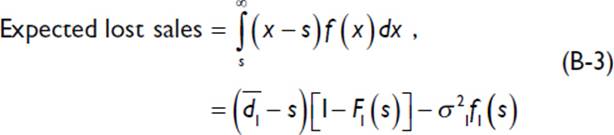
If the expected demand for the first period is d1 and the forecast error is σ1, stocking s units of supply yields the following value for lost sales in the first period:
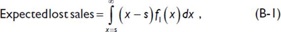
where x represents the random demand variable. It is possible to simplify the Equation B-1 by applying the following identity for a normally distributed density function:
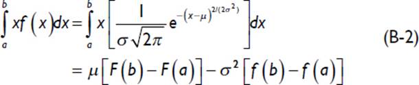
Plugging this identity into Equation B-1 results in an expression for lost sales that is directly related to demand characteristics—namely, the expected demand and variability.
![]() Note These distribution terms are easily computed in a spreadsheet: The Microsoft Excel functions for these terms are:
Note These distribution terms are easily computed in a spreadsheet: The Microsoft Excel functions for these terms are:
![]()
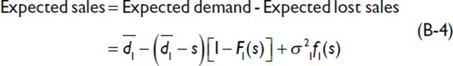
Having derived an expression for the expected lost sales, it is easy to compute the expected sales:
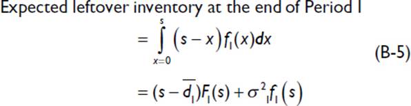
The expected leftover inventory at the end of the first period is calculated from the probability of supply exceeding demand according to the following relationship:
These single-period estimates need to be modified for multiple periods. The first estimate is the expected leftover inventory at the end of the second period, based on combining the demand probability distributions of the first and second periods, as follows:
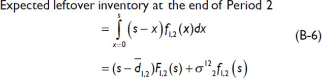
Equation B-6 assumes that demand across the two periods is independent. This is a reasonable assumption in many but not all situations. For example, if demand has decreased because the competition launched a better product, the uncertainties are likely to be biased for consecutive periods. However, many such situations can be effectively addressed by revisiting the demand forecast and generating new values based on such changes.
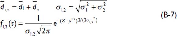
The combined probability distribution is calculated according to the following relationships:
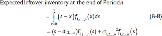
The same procedure can be extended to compute the leftover inventory at the end of the third and subsequent periods. If the product has a shelf life of n periods, the expected scrap inventory equals the leftover inventory at the end of the nth period, calculated as follows:
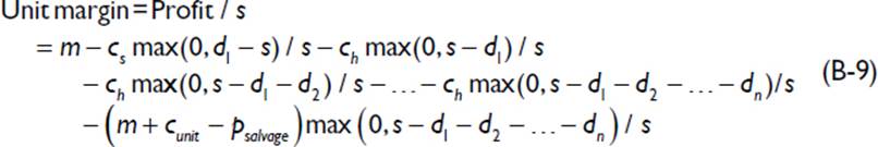
The expected margin from s units of supply is calculated subtracting shortage costs, holding costs, and scrap costs from the margin based on standard price and cost. The shortage cost is simply the cost of lost sales in the first period. The holding cost is the sum of the cost of holding inventory that is leftover at the end of the first and subsequent periods. Therefore, the expected unit margin can be written as follows:
The multi-period estimates presented in this appendix enable utilization of the detailed derivations in Chapter 2 to calculate other measurements, such as revenue and expedited units.
________________
1For the full derivation, see P. Mileff and K. Nehez, “An Extended Newsvendor Model for Customized Mass Production,” Advanced Modeling and Optimization, Volume 8, Number 2, 2006.