The Profitable Supply Chain: A Practitioner’s Guide (2015)
Chapter 4. Supply Planning
Supply planning is the process of specifying production and inventory levels in order to meet projected demand. It is a fundamental step for all goods-producing companies, and has been performed in one form or other since the advent of mass production. The reorder point (ROP) approach, still in vogue today, has been practiced since the industrial revolution. The Toyota Production System (TPS), introduced in the 1950s, was a revolutionary approach that helped rethink the flow of materials in a factory. The next development of note was material requirements planning (MRP), developed in 1964 by Joseph Orlicky. MRP is a rigorous demand-driven approach to coordinating material requirements across finished goods, sub-assemblies, and raw materials. The advent of advanced planning systems (APS) in the 1990s helped address some of the drawbacks of MRP, especially related to multisite production facilities and capacity constraints.
A drawback present in all supply planning systems is that they make several assumptions related to supplier operations, including production capacity and the time taken to manufacture. As supply chains have become leaner, planners have found that several of the issues adversely affecting supply plans are attributable to incorrect estimates of supplier operations. These issues are addressed by collaborating with suppliers to share plans and gain an understanding of suppliers’ real constraints. However, there are no uniform formal processes for company–supplier collaboration, and a supplier that sells product to several customers may have to collaborate according to very different processes and formats. One of the objectives of this chapter is to provide a process framework for collaboration that the author has developed based on his work with several large manufacturers.
The Importance of Supply Planning
For a company that sells products, the importance of ordering supplies in a timely manner to ensure adequate inventories is paramount. Consider the following quote from an annual report of Lowe’s, the home improvement company, about this topic:
Our financial performance could suffer if we fail to properly maintain our critical information systems or if those systems are seriously disrupted: An important part of our efforts to achieve efficiencies, cost reductions, and sales and cash flow growth is the identification and implementation of improvements to our management information systems to improve operations such as inventory replenishment systems, merchandise ordering, transportation, and receipt processing. Our financial performance could be adversely affected if our management information systems are seriously disrupted or we are unable to improve, upgrade, maintain, and expand our systems.
—Lowe’s Companies Inc., 2013 Annual Report
Indeed, inventory planning and demand planning both require the final step of replenishment and supply for execution of the plan. This chapter addresses the following questions:
· What is the quantity that needs to be ordered for a particular product at any given time?
· How can inventories at distribution centers be taken into consideration while creating production schedules at manufacturing plants?
· How can demand be used to drive orders for raw materials?
· How can the coordination of activities with suppliers be improved?
There are three types of models for generating supply orders—replenishment, requirements planning, and constraints-based planning. Replenishment models generate orders for a single item based on a fixed order quantity (continuous review replenishment) or a fixed interval for review (periodic review replenishment). Requirements planning models consider linkages between inventory and demand at various stages in the supply chain in order to determine order quantities. Examples include MRP and distribution resource planning (DRP). Constraints-based planningmodels build on requirements planning but add capabilities related to constraint identification and resolution. These three models are described in turn in the following sections.
The Supply Planning Process
The supply planning process is often managed by the manufacturing department of a company. The main functions of supply planning are:
· Requirements planning. The steps to convert the demand plan into a production and purchasing signal, considering on-hand inventories, production and transportation lead times, production capacity, and safety stock targets.
· Supply collaboration. The activities related to communicating the supply plan to key suppliers, and the subsequent exchanges to ensure that the schedules can be supported by the supplier in a timely manner.
The flow of information and interactions between the various steps is shown in Figure 4-1, for a company that relies on requirements planning for generating the supply plan. This procedure needs to be modified to suit a company’s specific needs. For example, a company with several manufacturing plants needs to introduce a step in which the plant managers review the production plans and decide whether production needs to be off-loaded from one plant to another based on capacity and other considerations.
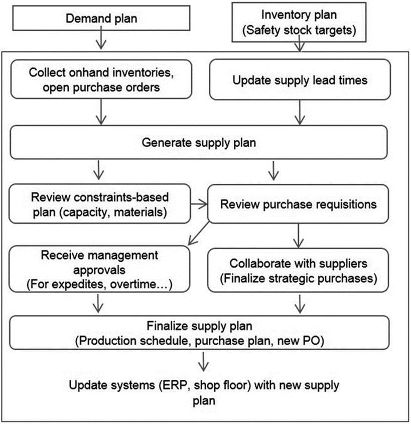
Figure 4-1. The supply planning process
Replenishment Models
Replenishment models are of two types—continuous review or periodic review. Continuous reviews result in a reorder at the instant when inventory levels reach a certain level, called the reorder point. Periodic reviews evaluate inventory position at specific intervals in time and inform the placement of orders to attain a target inventory level.
Continuous Review Replenishment
The continuous review model is often denoted as the (r, Q) policy, where r is the reorder point and Q is the reorder quantity. In many situations, Q is determined as the economic order quantity (EOQ), discussed in Chapter 2.
Once the EOQ and the safety stock target have been determined, the reorder point is calculated by Equation 4-1.
![]()
The use of a system to monitor inventories and trigger orders when the reorder point is reached will result in an average on-hand inventory calculated by Equation 4-2.
![]()
The duration between shipments is calculated by Equation 4-3.
![]()
Example 4-1 describes these calculations in detail.
EXAMPLE 4-1: AN ILLUSTRATION OF THE (R, Q) CONTINUOUS REPLENISHMENT POLICY
The demand forecast for a product is 100 units per week, and the forecast error is 20%. Supply variability can be ignored. A 98% service level is desired, and the supply lead time is 2 weeks. The company determines that the economic order quantity is 400 units.
Determining the Reorder Point
The safety stock is determined using the Service Level method for the 2-week lead time to be (2.06 * 20 * ![]() ) = 58 units (where 2.06 is the factor for the 98% service level). The reorder point is calculated from Eq. 4-1 as follows:
) = 58 units (where 2.06 is the factor for the 98% service level). The reorder point is calculated from Eq. 4-1 as follows:
Reorder point = Demand over lead time + Safety stock
= 2*100 + 58 = 258 units.
The average inventory is calculated to be (400/2 + 58) = 258 units, and the duration between shipments is (400/100) = 4 weeks. The anticipated inventory profile is shown in Figure 4-2.
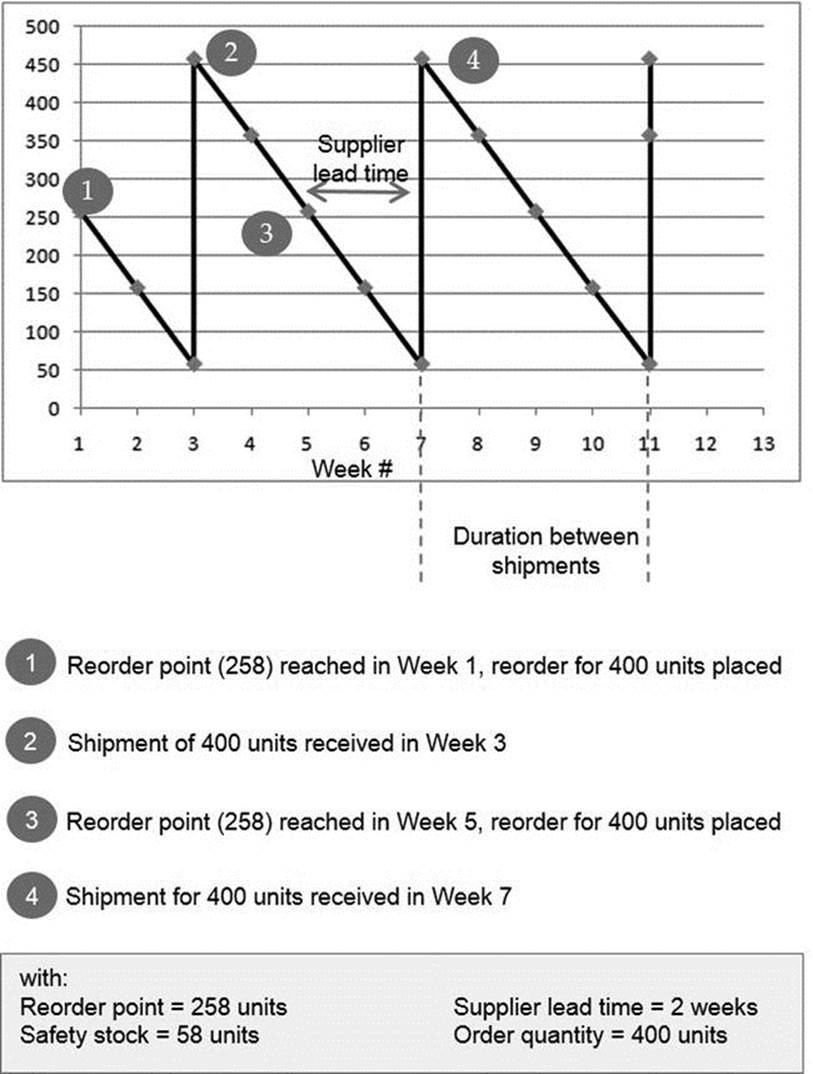
Figure 4-2. An illustration of continuous review replenishment
Periodic Review Replenishment
The periodic review model is often denoted as the (t, S) policy, where t is the review interval and S is the order upto level (OUL). The lead time is modified to include both the supply lead time and the review interval,
![]()
Usually, S is determined based on attaining a target service level according to the formula,
![]()
The average order size is calculated by the identity,
![]()
Since the total lead time is greater than the lead time for supply, the average inventory held in a periodic review system will be greater than in a continuous review system. The average inventory is calculated by the formula,
![]()
Because orders are initiated upon review, the duration between shipments is the review interval. Example 4-2 describes these calculations in detail.
EXAMPLE 4-2: AN ILLUSTRATION OF THE (T, S) PERIODIC REVIEW POLICY
For the data provided in Example 4-1, the review period is monthly (assumed for convenience to be 4 weeks). As a result, the total lead time is 6 weeks. The safety stock required is determined using the service level method to be (2.06 * 20 * ), or approximately 100 units. The order upto level is calculated as
Order upto level = Demand over lead time and reorder interval + Safety stock
= 6*100 + 100 = 700 units.
The average order size is the expected demand over 4 weeks = 400 units, and the average on-hand inventory = (400/2) + 100 = 300 units. An example of the inventory profile corresponding to this policy is shown in Figure 4-3.
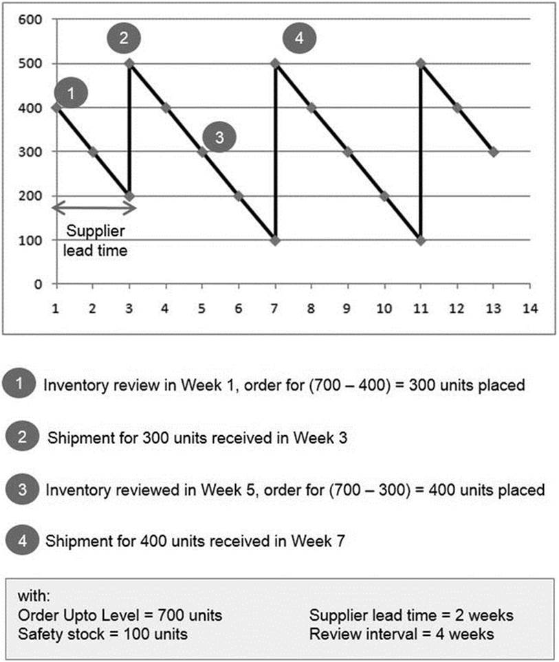
Figure 4-3. An illustration of periodic review replenishment
The guideline for the method to be used is based on the nature of the material being ordered. The (r, Q) reorder point policy is often used for short lead time, low-value orders since a manual review is often not necessary. On the other hand, the (t, S) periodic review policy is used for long lead time, strategic, or expensive items, and for capacity-constrained situations. In either case, when demand is not even and displays seasonality or varying prices and costs, it is necessary to recalculate safety stocks and economic batch sizes and adjust replenishment parameters accordingly. This is a reason for the popularity of sophisticated advanced planning systems that provide support for ordering based on future demand, costs, inventory control limits, capacity constraints, and transportation mode options.
Requirements Planning Models
Ordering supplies for material and parts whose demand depends on the demand for one or more other products is performed using requirements planning. Requirements planning can be applied to manufacturing and distribution situations. When applied to manufacturing, it is termed MRP, whereby finished goods and raw material inventories are considered together for the purposes of purchase ordering. The distribution situation is called DRP, whereby central and regional inventories are considered together.
Materials Requirements Planning
MRP converts a production schedule for products into time-phased requirements for subassemblies and parts, which, in turn, are converted into orders based on lead time, on-hand inventory, scheduled receipts, and inventory targets. The inputs required by MRP include the following:
· Master production schedule (MPS). The MPS specifies the production schedule for each of the product, and is calculated based on actual customer orders as well as demand forecasts.
· Bill of materials (BOM). The BOM specifies the amount or number of raw materials, components, and sub-assemblies needed to manufacture each product.
· Item master. This file specifies item characteristics, including lead time for production or purchasing, as well as target inventories.
· On-hand inventory. The on-hand inventory for each of the specified items is required for netting requirements.
· Scheduled receipts. For long lead time items, scheduled receipts need to be tracked and used for netting requirements.
The requirement on each part is referred to as dependent demand, while product demand is referred to as independent demand. The difference between these two is that independent demand is calculated using the forecasting or consensus methods described in Chapter 3, whereas dependent demand is calculated from the independent demand (hence the use of the term “dependent”). The steps in the calculation are:
· Explosion. Demand or the production schedule is converted to component requirements (quantity and schedule) using the BOM. If a part is used in multiple bills, the requirements from the individual products are added together. Inventory targets are specified as a quantity or as time, and are included in the requirements.
· Netting. Any on-hand inventory is subtracted from the requirements calculated from the previous step. When there are multiple manufacturing steps (for example, when subassemblies are created from raw material, and in turn, used to manufacture products), netting needs to be performed for each of these subassemblies considering on-hand and work-in-process (WIP) inventory. WIP inventory represents inventory of products or subassemblies that is in the process of being converted from its raw to finished form.
· Offsetting. This step incorporates lead times into the schedules, in order to determine the timing of supplies. For subassemblies, the lead time for production is used; for raw material, lead time for supply is used.
When there are multiple manufacturing steps, these calculations are performed for each in an iterative manner, from finished goods to subassemblies to raw materials. Example 4-3 illustrates these steps.
EXAMPLE 4-3: AN ILLUSTRATION OF MATERIALS REQUIREMENTS PLANNING
Data for MRP for an electronics company is provided in Figure 4-4, including the item master, bill of materials, on-hand inventory, scheduled receipts, and independent demand.
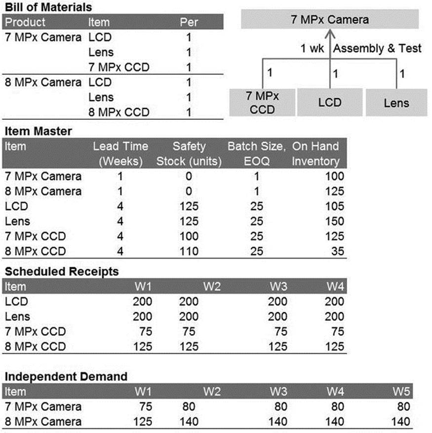
Figure 4-4. Materials requirements planning (MRP) data) for Example 4-3
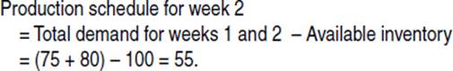
The first step is to calculate the production schedule from the independent demand for each of the products, as shown in Figure 4-5. In this calculation, the production schedule is calculated by subtracting the cumulative value of inventory and production from the cumulative value of demand for the previous weeks. For example, the production schedule for week 2 is calculated as
Supply requirements for parts are calculated based on the production schedule for the finished good and the lead time for production. The procedure for calculating requirements depends on whether each is used by one or both products; when a part is used by only one product, the requirement is calculated by simply offsetting the production schedule by the appropriate lead time, as shown in Figure 4-5 for the 7MPx CCD part.
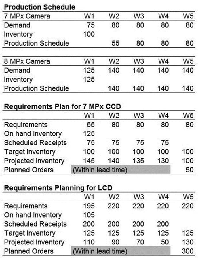
Figure 4-5. Production schedules and requirement plans for Example 4-3
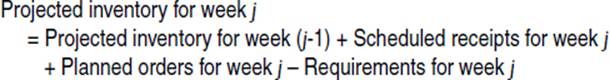
In the figure, the projected inventory for the end of week j is calculated according to:
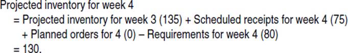
For example, the projected inventory for week 4 is calculated as
Planned orders for a period are calculated based on meeting a target inventory (i.e., safety stock):
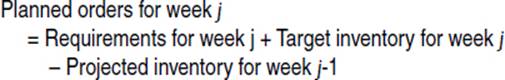
Therefore, the planned orders for week 5 are
Planned orders for week 5 = 80 + 100 – 130 = 50 units.
Note that the planned order quantity may need to be modified based on the lot size specified. Since the lot size for the part is 25 units (from the Item Master data table), no modifications are necessary. If the lot size had been 30 units, then the planned order is rounded to the closest multiple, i.e., 60 units. These additional 10 units would result in an inventory level in excess of the target.
When a part is used across multiple products, requirements need to be calculated based on the production schedules for each of the products, time-phased by the appropriate lead time. In this example, the LCD part is utilized by both camera products (as shown in the BOM). The procedure for calculating LCD requirements is shown in Figure 4-5.
The requirements are calculated by adding the combined production schedule for the 7 and 8 MPx cameras. Since production lead times are identical for both products, the schedules for the same weeks can be added (for example, week 2 requirements of 220 units are obtained by adding 80 and 140 units for the 7 MPx and 8 MPx cameras, respectively). Once these combined requirements have been calculated, the procedures for computing projected inventory and planned orders are identical to the previous situation.
MRP has been adapted to deal with several other situations, such as manufacturing yield, sub-assemblies, and engineering changes.
There are several situations that may require the procurement organization to issue purchase orders that are different from the quantity dictated by the MRP bill-of-material explosion). Examples of such situations include:
· Price discounts from the vendor for bulk purchases that have not been accommodated by the lot size specification.
· Early purchasing in anticipation of a price hike or an industry-wide material shortage.
· Deferred purchasing in anticipation of a price reduction.
These situations require the materials planner to modify the MRP output and adjust order quantities as needed.
Distribution Requirements Planning
Replenishment models are frequently used to order material at distribution centers, which works well for single stage distribution networks. However, companies supporting a wide geography often rely upon a distribution network consisting of central distribution centers that feed local facilities (see Figure 4-6); in such cases, inventories need to be coordinated across the distribution network, achieved by DRP. The data requirements for DRP are similar to MRP and include:
· The independent demand forecast for each product at the respective distribution centers.
· On-hand inventories.
· Target safety stock.
· Transportation lot sizes or economic replenishment quantities.
· Replenishment lead times and frequencies.
Since the logic used to convert demand into requirements and replenishment orders is identical to MRP logic, an MRP system is often used to perform DRP. For manufacturing companies, the output of DRP is the demand that is placed on the manufacturing plants and is used to drive MRP. Example 4-4 illustrates the use of DRP.
EXAMPLE 4-4: AN ILLUSTRATION OF DISTRIBUTION REQUIREMENTS PLANNING
The distribution network for a consumer goods product is shown in Figure 4-6. Goods are manufactured overseas and shipped to the United States using ocean containers. The goods are imported at the Los Angeles port and inventoried at the central distribution facility in close proximity. This central facility is used to fulfill demand from retail customers in California and neighboring states. In addition, two regional distribution centers are maintained in Chicago, Illinois and Dallas, Texas to fulfill retail demand for the Midwest and Southwest regions, respectively.
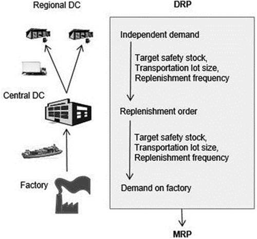
Figure 4-6. Use of distribution requirements planning (DRP) for a two-stage distribution network
The supply lead times for the regional distribution centers are 1 week, while the supply lead time for the central distribution center is 8 weeks, with a container size of 2,000 units. Safety stocks are set to 1 week for the regions and 3 weeks centrally. The independent demand for a product at these facilities is shown in Figure 4-7. With this information, the replenishment plan for each of the regions can be completed, shown in Figure 4-7 for the Midwest region.
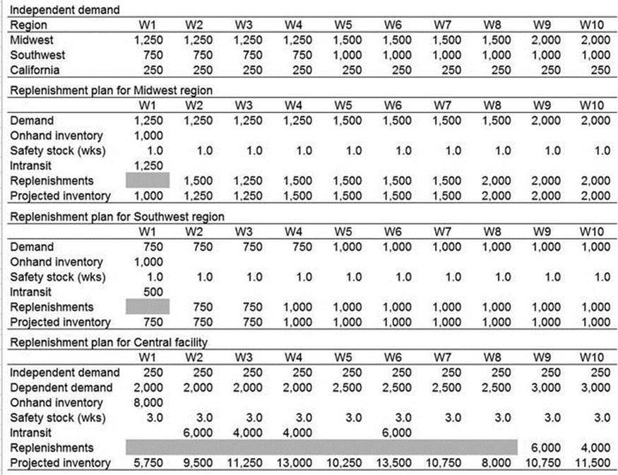
Figure 4-7. Distribution requirements planning (DRP) calculations for Example 4-4
The first four rows (demand, on-hand, target safety stock, and in-transit) are inputs to DRP. The calculations for the end of week (ending on-hand or EOH) projected inventory and replenishments are similar to the MRP calculations. The projected inventory for the first period is calculated as (on-hand + in-transit – demand) = (1,000 + 1,250 – 1,250) = 1,000 units. Next, the replenishments for week 2 are calculated as
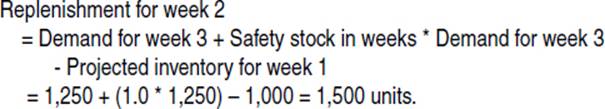
Note that the second term in the equation is the calculation to convert safety stock from weeks to units, and, in this example, is based on providing inventory cover for demand for the following week (i.e., week 3). The replenishment for the Southwest region is performed in a similar manner, shown in the second section in Figure 4-7.
The procedure for the central facility is different due to two streams of demand—the first is the independent demand for the California region and the second is the dependent demand from the two regions. Since there is a 1-week lead time to the regions, the dependent demand is placed one week earlier on the central facility. Additionally, since the central facility is replenished via ocean shipments with a lot size of 2,000 units (container load) and an eight week lead time, no replenishments can be arranged in the first 8 weeks. This 8 week window is shown in gray in the Replenishment row.
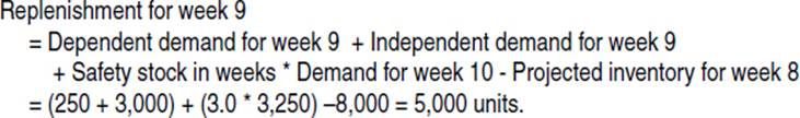
Note that the requirement of 5,000 units is rounded up to 6,000 due to the 2,000 unit lot size. The replenishment requirements into the distribution center will act as the production requirements to be placed on the manufacturing facility. Therefore, for companies that operate manufacturing plants and distribute products in several regions, the workflow will involve a DRP run, followed by an MRP and production scheduling run.
DRP allows for the inventory picture across the entire network—on-hand and in-transit—to be considered while planning supplies. This coordinated view across the network ensures that inventories are in line with targets.
Constraints-Based Planning
A constraint is any factor in the supply chain that limits output and hinders attainment of the targeted goals. Examples of constraints are inadequate manufacturing capacity and insufficient storage space for inventory. One of the drawbacks of MRP and DRP is the inability to deal with a wide variety of constraints—both provide a simple approach to capacity and lead times, sometimes resulting in plans that do not provide the company with the desired output. The need for constraints-based planning is best understood by way of an example. Consider the distribution plan for the central region in Example 4-4. What if the beginning on-hand inventory were not 8,000 units but only 100 units? The requirements would look quite different since the projected inventory calculation would result in negative values, indicating insufficient inventory in weeks 1 and 8, since the lead time for ocean transit does not allow for a shipment to be received until week 9. This mismatch between demand and available and planned supply is a constraint since it does not allow the supply chain to perform as desired.
A common constraint situation involves insufficient manufacturing capacity. The options available to resolve this issue are to authorize overtime in order to increase output, prebuild inventory when sufficient lead time exists, or change product mix in case product inventories permit. Selecting the right option is not a trivial task. Not only do companies need to evaluate the feasibility of each option—for example, will changing the product mix reduce output due to higher setup times?—but they also need to analyze the cost implications. Table 4-1 provides a few examples of constraint situations and resolution options.
Table 4-1. Examples of Constraints and Resolution Options
|
Constraint |
Resolution Options |
|
Insufficient capacity |
Authorize overtime for production workers. Prebuild inventory in prior weeks when capacity is available. Change production mix to balance finished goods inventory. Offload production to another plant. Outsource production of commodity products. |
|
Insufficient raw material inventory |
Expedite materials using alternative transportation modes (e.g., air shipment vs. ocean). Use alternative supplier with lower lead times. Use alternative parts that can meet specifications. |
|
Insufficient distribution inventory |
Expedite materials using alternative transportation modes. Source goods from an alternative manufacturing plant. Source goods from another distribution center. |
Capacity Constraints Due to Seasonal Demand
Managing inventory during peak demand periods is a challenge faced by all consumer goods companies. Examples of peak demand periods include Christmas, back-to-school, and Halloween. Consider the following excerpt from an annual report of an apparel retailer:
The retail apparel market has two principal selling seasons, Spring (first and second fiscal quarters) and Fall (third and fourth fiscal quarters). As is generally the case in the apparel industry, the Company experiences its greatest sales activity during the Fall season. This seasonal sales pattern, in which approximately 40% of the Company’s sales are realized in the Spring season and 60% in the Fall, results in increased inventory during the Back-to-School and Holiday selling periods. During Spring of Fiscal 2005, the highest inventory level of approximately $364.0 million at cost was reached at the end of July 2005 and the lowest inventory level of approximately $211.2 million at cost was reached at the beginning of February 2005. During Fall of Fiscal 2005, the highest inventory level of approximately $418.5 million at cost was reached at the end of November 2005 and the lowest inventory level of approximately $342.3 million at cost was reached at the end of December 2005.
—Abercrombie & Fitch, 2006 Annual Report
Clearly, the large difference in sales through the year places an enormous strain on manufacturing operations, and companies are forced to take on inventory positions that depend on the forecast, manufacturing capacity, cost of production using overtime labor, and cash positions. This mismatch between capacity and demand is illustrated in Figure 4-8 for a consumer product that displays significant demand in two to three months of the year. In addition, service level and safety stock calculation can further exacerbate the situation, as shown in the middle graph in Figure 4-8. In most situations, the required production levels can far exceed the capacity of the manufacturing plants, as shown with the two horizontal lines representing shift-based production capacity.
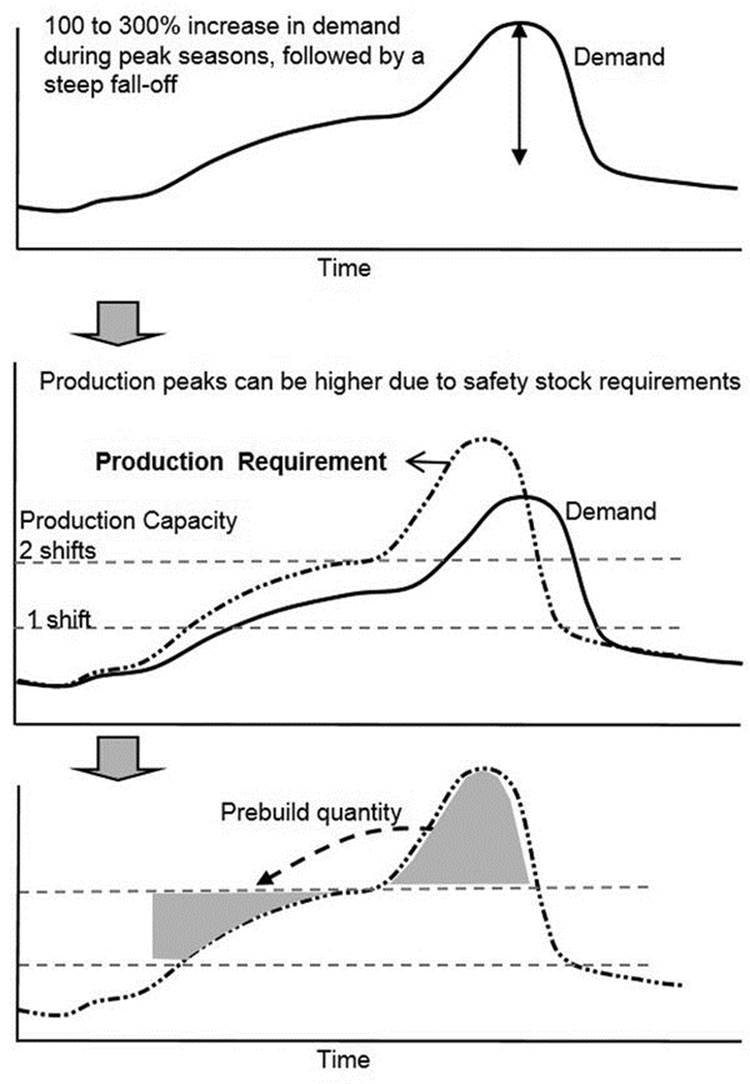
Figure 4-8. Meeting seasonal demand peaks by building ahead
Adding capacity is not a desirable option due to the low utilization during the off-season. Furthermore, even if tooling investments were made, the ability to adjust the labor force according to the peaks may not be possible. Instead, an alternative option is to build additional inventory during the lean periods leading up to the season, and building to capacity during the peak season. This strategy provides the additional benefit of increasing utilization in the earlier periods. The resulting prebuild inventory is illustrated in the bottom graph in Figure 4-8.
The additional inventory that accumulates as a result of this action is referred to as seasonal or prebuild inventory. While it allows manufacturing plants to meet market demand without additional tooling investments, the strategy is not without a disadvantage since it increases inventory holding costs. When penalties associated with holding inventory are high, for example if obsolescence is a consideration, other options can be evaluated, such as the use of lower-cost warehouses for storing inventory, selling goods earlier to channels, or striking deals with channel partners to share a portion of any increased costs.
Seasonal demand may not be the only reason for accumulating prebuild inventory. The need can also arise when multiple products consume the same production resource at a manufacturing plant. Since capacities are usually set based on anticipated demand, a favorable situation when demand simultaneously increases for some or all of the products can result in a constrained situation at the manufacturing plant. If production capacity is lesser than the anticipated demand, the need to accumulate inventory arises. Example 4-5 illustrates a prebuild analysis.
EXAMPLE 4-5: PRODUCTION PLANNING FOR A PRODUCT EXPERIENCING SEASONAL DEMAND
Requirements and capacity for a consumer good, along with prebuild calculations, are given in Figure 4-9. The Capacity Shortfall row in the first illustration (the difference between requirement and capacity) shows that capacity is inadequate in months 5 and 6. Using this information, there is a simple method for calculating prebuild quantities. The first step is to calculate available capacity and shortfalls for each of the months, as shown in the Capacity Available row in the second illustration in Figure 4-9.
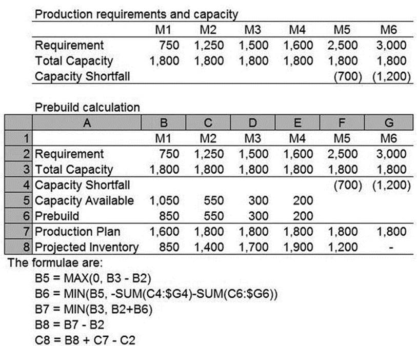
Figure 4-9. Input data and prebuild calculations for Example 4-5
Once capacity availability and shortfalls have been calculated for each month, prebuild quantities are calculated in reverse order—the first calculation is performed for the month immediately preceding the shortfall (i.e., Month 4) using the formula shown at the bottom of the figure. Once the prebuild quantity for Month 4 has been completed, the procedure is repeated for Month 3 until the entire shortfall has been covered. Due to this reverse traversal, the resulting production plan is optimal since it minimizes the buildup of inventory.
Once prebuild quantities have been determined, the production plan is calculated for each month as the sum of the requirement and prebuild quantity for that month. Finally, the projected inventory is simply the difference between total production and the requirement for that month. The numbers clearly show the build-up of inventory in the first 4 months, which is consumed by the seasonal demand in months 5 and 6.
When multiple products are produced using the constrained resource, an additional decision needs to be made regarding the specific product that should be prebuilt. Some of the considerations for this decision are:
· Availability of raw material. Prebuild requires that raw material inventory also be available at an earlier time.
· Availability of storage. If storage space is limited, storage capacity will need to be considered.
· Minimizing exposure. If product demand is uncertain, it is necessary to evaluate the additional exposure due to prebuild inventory.
It is natural to prebuild the product with higher volume and greater margin first, since the additional inventory can be sold for a greater profit. While this is generally accurate, another factor that companies need to take into consideration is the holding and obsolescence cost—products with high price erosion or holding costs are not good candidates for earlier production. Once the priority of products to be prebuilt has been determined, the production plan for each of the products in the earlier periods needs to be calculated. The simple method shown in Example 4-5 for a single product can be extended to analyze several products. However, when the number of products is large and additional factors need to be considered (for example, raw material availability), the use of heuristic methods or linear programming becomes necessary. Many advanced planning systems provide such capabilities.
Advanced Planning Systems
The section on requirements planning has shown how materials can be planned for the manufacturing and distribution sections of the supply chain separately. However, the resulting workflow for a company that operates several facilities requires significant coordination and is a daunting task. In addition, support for resolving constraints is minimal, and requirements planning systems leave much of the problem solving to the production scheduler or purchasing agent. These issues have resulted in the adoption of advanced planning systems (APS) for complex multi-facility supply chains. When properly implemented, these systems can have a significant impact on margins, as observed in an annual report by Adtran, a manufacturer of networking and communications equipment:
Cost of sales, as a percentage of sales, decreased from 42.9% in 2004 to 40.9% in 2005. The decrease is primarily related to manufacturing efficiencies, the timing differences between the recognition of cost reductions and the lowering of product selling prices, and the sales of higher margin new products. In addition, the decrease resulted from improvements in supply chain management, due to the implementation of an advanced planning system and a web-based procurement process, which has reduced cycle times and increased our manufacturing flexibility. We anticipate that continued deployment of supply chain applications augmented with process improvement strategies will result in further cost reductions, which we believe will provide a continued competitive advantage.
—Adtran, Inc., 2006 Annual Report
The importance of advanced planning systems is also emphasized by a furniture manufacturer, Steelcase.
The Company manufactures its products at more than 30 locations throughout the world, including the United States, Canada, Mexico, and Europe. In 1987, the Company adopted world class manufacturing principles which utilize a variety of production techniques, including cell or team manufacturing, focused factories, and rapid continuous improvement. This initiative has evolved to include advanced planning and scheduling systems and is referred to as the Steelcase Production System. The Company continually examines new opportunities to consolidate its manufacturing and distribution operations to improve efficiency. Substantially, all plants “build to order” rather than to “forecast,” which directly reduces finished goods inventory levels and emphasizes continuous improvement in set-up and delivery time to customers. As a result of these and other order processing and customer service improvements, the Company’s average lead-time, i.e., the time from order to delivery, has been reduced in the United States and Canada.
—Steelcase Inc., 2013 Annual Report
The excerpt indicates that the cost of implementation of such systems is significant; however, companies still see sufficient financial benefit and return on investment from such a system. Yet another example is from an annual report of Paccar, a commercial vehicle manufacturer:
Leyland operates one of the most efficient truck factories in the world. The 710,000-square-foot plant incorporates an innovative robotic chassis paint facility and a state-of-the-art Advanced Planning and Scheduling system to produce DAF’s entire LF, CF and XF product line. This complex mix of vehicles—with its widely different market requirements—serves customers in Europe, Australia, Africa, and North America.
PACCAR was selected as a “Supply Chain Top 25” leader by AMR Research because of the integration of its global supply chain. PACCAR’s Dynacraft supply chain management services developed a global advanced-planning system that shortens truck production scheduling from hours to minutes, and implemented state-of-the-art chassis robotic paint software to realize manufacturing efficiency and product quality benefits.
—Paccar Inc., 2007 Annual Report
Clearly, companies across many different industries see a significant advantage in implementing advanced planning systems. Some of the capabilities provided by advanced planning systems include:
· Support for coordinating activities across multiple sites. When a company operates multiple distribution centers and manufacturing plants, APS calculates requirements for the distribution centers and converts the necessary replenishments into dependent demand for the manufacturing plants.
· Explicit handling of constraints. One of the ways that advanced planning differs from traditional requirements planning is by simultaneously considering material and capacity, which results in more realistic plans. When demand is in excess of capacity, APS can consider several alternatives, including alternative line capacity and even available capacity at alternative facilities. When material is short, alternative parts or suppliers can be considered. When the mismatch is due to transportation schedules, alternative modes of transport can be considered. This general approach toward constraint resolution is a significant benefit provided by APS.
· Provision for collaborative workflows. The resolution of constraints becomes harder to analyze and execute in an outsourced supply chains since it is harder to collect information in a timely manner and understand the true capability of the supply chain. For this reason, collaboration has become an increasingly important process and is an important feature provided by advanced planning systems. Collaborative workflows are expanded on in the following section in this chapter.
· Creation of feasible plans. When constraints cannot be resolved, the resulting mismatch between supply and demand needs to be resolved by ensuring that scarce resources are utilized in the best possible manner. This process of allocation is expanded on in the discussion of sales and operations planning in Chapter 5.
· Ability to evaluate network options. Along with planning requirements across multiple facilities, APS need to incorporate features that allow the analyst to evaluate improvements that are possible by alternative routings and alternative placement of facilities. Details regarding such analyses are provided in the discussion of network planning in Chapter 6.
· Support for a performance review process. The calculation of metrics and support for what-ifs requires not only the incorporation of financial information, but also the capability to re-plan quickly and address the different kinds of questions that can arise. Details regarding the performance review process are provided in Chapter 7.
Advanced planning systems employ one or more methods for constraint resolution, including heuristics and linear programming. A heuristic is a problem solving method that utilizes rules or educated guesses in order to arrive at a good answer. When applied to planning supply, heuristics consist of a series of steps for evaluating alternatives, as shown in Figure 4-9 and illustrated in Example 4-5. Heuristics have gained popularity since they can be easily understood and programmed. However, heuristics cannot be mathematically proven to arrive at an optimal solution; therefore, they need to be used with care. Complex supply chains involving constraints at multiple manufacturing and distribution stages are typically hard to tackle using these methods.
An alternative to the use of heuristics is linear programming (LP). LP refers to a mathematical technique for optimizing a set of linear objective functions subject to linear constraints.1 LP is better suited than heuristics for arriving at optimal solutions for complex problems. However, it is not without shortcomings—defining LP models requires skill, and nonlinearities such as lot sizing (for manufacturing or transportation) cannot be included in the model. Due to this limitation, it is often necessary to solve the problem using LP to arrive at a specific production plan, and to modify this plan using heuristics to accommodate nonlinear constraints. Since there is a reliance on heuristics, the final solution is not guaranteed to be optimal and the production and distribution plan can result in excess inventories for certain parts and products, and simultaneously an inability to satisfy demand for other products.
Since there is no single approach that performs adequately for all situations, it is necessary for the analyst to gain an understanding of the specific method being utilized by the planning system in order to identify situations that can result in suboptimal production. If such situations are encountered, manual intervention is needed to perform additional checks or procedures to improve efficiency. Examples of guidelines that can be used during exception resolution are shown in Table 4-2.
Table 4-2. Sample Guidelines for Exception Resolution
|
Product Characteristics |
Resolution Guidelines |
|
Variable demand, steady price, high margins |
Maintain high service levels. For example, consider use of multiple modes of transportation to meet demand. |
|
Variable demand, steady price, low margins |
Limit margin erosion by tightly managing supplies (e.g., ocean freight only, no overtime labor). Service levels may be sacrificed. |
|
Variable demand, decreasing prices and margins (lifecycle products) |
Evaluate use of mixed strategy: maintain high service levels initially (e.g., use local manufacturing, air freight), but limit margin erosion toward end-of-life. |
Advanced planning systems are not without their disadvantages—they are complex, time consuming, and not guaranteed to resolve a problem in the best possible manner. However, the alternative is to rely solely on human effort and insight, which can prove to be costly when the staff is inexperienced or when supply chains are complex and involve numerous products. In such situations, the benefit of APS is undeniable, especially when used in a decision-support mode.
Supply Collaboration
In an increasingly outsourced supply chain, there is a clear need for collaboration between partners to ensure visibility and alignment of demand and supply. Supply collaboration can provide early visibility to suppliers regarding changes in demand and purchase schedules, and provide buyers with visibility to shipping schedules and changes. The Beer Game, developed at MIT in the 1960s, demonstrates the value of sharing information across the different entities in a supply chain.2 This instructive exercise clarifies how each entity, acting in isolation, can increase costs for the entire supply chain.
While it is impossible to react immediately to changes in demand, especially with the extended lead times in outsourced supply chains, the magnitude of the inventory charge may have been reduced by better visibility and reaction across the supply chain. No doubt this example is egregious, but day-to-day supplier operations and misalignment impact costs in less extreme but nevertheless significant ways.
Several companies have realized that collaboration is valuable and a few early examples deal with the standardization of the process between a manufacturer and a retailer—referred to as Collaborative Planning, Forecasting, and Replenishment (CPFR), described in Chapter 3. Since CPFR is geared toward information related to retail sales and promotions, it is not directly applicable to communication with suppliers. Instead, different procedures are required, with additional focus on capacity and schedules. The most common collaborative processes between a manufacturer and suppliers are:
· Purchase order collaboration. The communication of purchase order (PO) and shipment details, and alerts when quantity variances or schedule changes occur.
· Inventory collaboration. The communication of demand and on-hand inventory information required to support a vendor-managed inventory (VMI) situation.
· Supply forecast collaboration. The communication of product or product-group level requirements in order to provide the supplier visibility to future order quantities.
· Capacity collaboration. Of special importance when custom parts are being purchased, the communication of capacity information ensures that the right product-mix decisions are taken.
Figure 4-10 summarizes these exchanges for two trading partners.
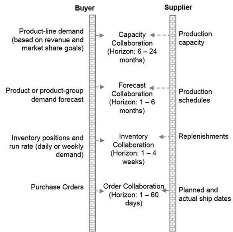
Figure 4-10. Examples of collaborative processes
Purchase Order Collaboration
Purchase orders may be initiated several weeks to months ahead of the receipt of goods, depending on the lead time for supply and transportation. During this time, it is possible for quantities, delivery dates, destinations, and prices to change, which can adversely impact manufacturing schedules and customer deliveries. The goal of purchase order collaboration is to reduce the occurrence of such variances.
The information communicated and tracked by this process includes order details as well as information such as the following that can be used to avert delays:
· Transactional information, including the order number, header information, lines, quantities, and schedules.
· Tracking information related to the order communication date, supplier acknowledgment date, and shipment and receipt dates.
· Supporting and alerting information, including dates and reasons for schedule changes.
Software enabling this collaboration triggers alerts when shipments are not made and goods are not received according to schedule. Such tools can greatly reduce the manual effort required to monitor and manage issues.
Inventory Collaboration
The goal of inventory collaboration is to provide suppliers visibility to inventory levels at the buyer’s facilities in order to ensure timely replenishments. The most common application of inventory collaboration is to support the VMI process. VMI requires that the supplier monitor inventory levels and plan supplies in order to ensure that inventories remain at a specified level. Advantages of a VMI program include the following:
· Timely and accurate replenishments translate into revenues for the supplier, which is a strong incentive for ensuring that adequate attention is being devoted to the monitoring of inventory levels and supplies.
· The transfer of activities for reviewing inventory and placing purchase orders to the supplier frees up resources within the company, which eventually translates to cost savings.
· A VMI program is usually accompanied by a pricing agreement that does not favor large, lumpy supplies. As a result, the supplies can be better aligned with production capacity and the buyer receives consistent prices.
The basic information to be communicated includes on-hand inventory and on-order information. In addition, a view of future demand is provided in the form of weekly demand and demand over the replenishment lead time. Finally, supporting information, such as the criticality of the part for the production process, can help the supplier ensure adequate service levels.
Inventory collaboration is performed according to a specific schedule, usually daily or weekly. Frequent reviews will ensure a quick response in case of demand spikes. The use of a system reduces the effort required and provides the additional benefit of continuous monitoring and triggering of replenishments on an as-needed basis, if appropriate.
Supply Forecast Collaboration
When lead times are long, a lack of alignment between demand and supply can result in shortage situations lasting several weeks or months. In such cases, a signal in advance of the purchase order may help align demand with the supplier’s production capacity. Since the purchase order is binding, companies tend to delay its release until the last possible moment, when demand is clear and there is a high level of confidence that the purchases are necessary. On the other hand, the communication of a non-binding forecast can address these disinclinations and promote visibility across companies.
From a supplier’s perspective, visibility to forecast can be extremely useful for planning production. However, it is in the interest of companies to ensure that forecast accuracy is high; otherwise the suppliers will ignore these numbers and use internal forecasts instead.
The information requirements for forecast collaboration are relatively simple—at a minimum, the buyer needs to communicate the forecast quantities, while the supplier needs to communicate committed quantities. Any mismatches are highlighted and serve as the starting point for dialogs and resolution steps. Since new forecasts are generated during material planning, the frequency of communication is usually weekly or monthly.
Capacity Collaboration
Capacity collaboration is required when suppliers provide custom-designed parts, or use dedicated production lines or specialized tools to manufacture one or more products. The lack of readily available alternative sources requires that long-term demand and capacity be aligned, usually for the next 6 to 24 months. Therefore, the goals of capacity collaboration are to ensure that adequate manufacturing capacity exists at the supplier’s plant and that the right mix of products is being produced. Several factors can complicate capacity collaboration:
· The horizon for capacity collaboration is usually long, ranging from 3 to more than 24 months. The number of variables that can come into play in this time frame makes data collection challenging and requires reliance on forecasts that might exhibit high error.
· Manufacturing complexity related to multiple product-lines consuming the same resource, in order to leverage tooling investments. This complicates the collaborative process since it requires that many product managers collaborate, and that trade-offs between different options be considered.
· WIP tracking complexity, especially when the manufacturing process has several steps that take several days to complete.
An example of this analysis is shown in Figure 4-11. From the figure, it is clear that the information required by this process is more involved than the other situations, and includes, at a minimum, demand by product line and capacity information. In addition, a simple bill-of-consumption that specifies the capacity usage of the different product lines needs to be specified. With this information, a simple plan that identifies capacity shortfalls and resolution options can be generated and used for further analysis.
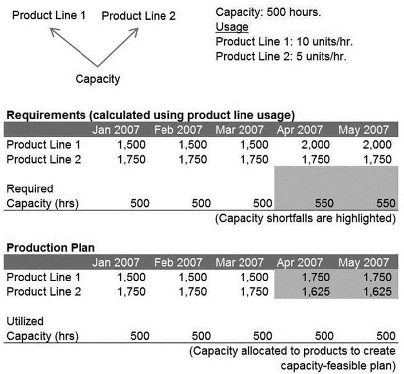
Figure 4-11. An illustration of capacity analysis
The collaborative workflows that a company should consider depend on the characteristics of the part being sourced. While custom-designed parts require the highest level of alignment and collaboration, commodity items may require only a limited exchange of information, as shown inFigure 4-12. Other factors that need to be considered include the cost of materials, lead times, easy available of alternative suppliers, and exacting quality requirements.
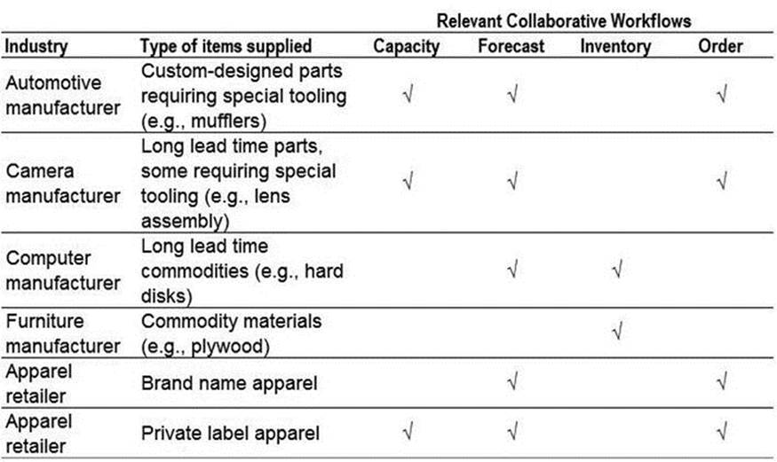
Figure 4-12. Guidelines for applicability of collaborative processes
Apart from the collaborative processes discussed above, additional information to be communicated may include situations related to new product introductions, expansions to new markets, and quality and testing procedures. While designing workflows and systems for these collaborative processes, it is important for business partners to have a clear idea of the information shared, communication schedules, and a clear action plan to deal with issues identified as a result of the collaboration.
Summary
This chapter introduced methods for managing supplies and purchases based on the guidance provided by demand planning and inventory planning. Replenishment models can be used to create orders for items when inventory reaches a particular level. These models are simple to use and easy to implement with systems, but do not perform well when demand is highly variable, or when inventories need to be coordinated across several points in the supply chain. Such coordination is required when finished goods are manufactured from sub-assemblies and parts, or when there are multiple stages of distribution with central and regional facilities.
Requirements planning models connect inventory across several items and parts as well as stages of distribution. Therefore, these models are effective for coordinating supplies across the supply chain, but they do not perform well when constraints occur; examples of constraints include insufficient inventory and insufficient capacity. These situations are better addressed by advanced planning systems, which provide connectivity across items and facilities in the supply chain and the ability to identify and partially resolve constraints. However, these systems are often complex and expensive to implement.
The importance of collaboration for the current business environment cannot be over-emphasized. Effective collaboration can reduce supply variability and reduce inventory levels. Therefore, it behooves every company to seriously consider one or more of the collaborative processes described in the chapter. Traditionally, electronic data interchange (EDI) has been the most prevalent method for exchanging information between companies. EDI is restricted in the richness of data that can be communicated, is expensive to customize, and does not provide any guidelines regarding the collaborative process and schedules.
As a result, several industry standards have been created in order to provide structure to collaboration. For example, the Voluntary Interindustry Commerce Solutions (VICS) Association has published guidelines for data required for CPFR. Building on standards that existed in EDI communication, the Electronic Business using eXtensible Markup Language (ebXML) specification was developed jointly by the Organization for the Advancement of Structured Information Standards (OASIS) and the United Nations Center for Trade Facilitation and Electronic Business (UN/CEFACT). The ebXML specification provides standards for supply chain data as well as business processes and collaborative protocol agreements.
In addition, industry-specific standards exist. For example, RosettaNet, a nonprofit association of companies, specifies several Partner Interface Processes (PIP) that provide data guidelines for the electronics industry. Each of these standards has been developed in order to address specific processes and data, though significant overlaps exist. It behooves companies to invest the resources needed to evaluate and settle on the specifications that are best suited for their products and business processes.
________________
1F. S. Hillier and G. L. Lieberman, Introduction to Operations Research (McGraw-Hill, 1997).
2Michael Hugos, Essentials of Supply Chain Management (John Wiley, 2003).