The Profitable Supply Chain: A Practitioner’s Guide (2015)

Chapter 3. Demand Planning

Demand planning is the process of understanding customer and market perceptions of the company’s products and specifying an accurate picture of future revenues and sales volumes. The benefits are easy to understand: good management of demand will help improve customer service and relationships, a paramount goal for most companies. An accurate forecast will also serve to align supply with demand, resulting in lower inventory and capacity levels and reduced waste and costs.

The availability of demand-related information has increased dramatically in this increasingly digital world, but courses and textbooks on demand planning still expound on traditional forecasting methods, mainly time series (i.e., forecasts generated based on sales history). But the forecaster is faced with challenging situations almost on a daily basis, from dealing with a cloudy economic outlook to gauging the impact of a competitor’s new product. Traditional forecasting methods provide little support for analyzing such needs.

This chapter addresses these needs by providing several approaches for understanding and handling non-standard situations, including price elasticity, economic indicators, expansion to new markets, the impact of weather, distortion of channel forecasts, and collaborating with channel partners.

The Importance of Demand Planning

The importance of accurate forecasts is emphasized in the following statements by Plantronics, a manufacturer of headsets for telephones.

We determine production levels based on our forecasts of demand for our products. Actual demand for our products depends on many factors, which makes it difficult to forecast. We have experienced differences between our actual and our forecasted demand in the past and expect differences to arise in the future. Significant unanticipated fluctuations in demand and the global trend toward consignment of products could cause the following operating problems, among others:

If forecasted demand does not develop, we could have excess inventory and excess capacity. Overforecast of demand could result in higher inventories of finished products, components, and sub-assemblies. In addition, because our retail customers have pronounced seasonality, we must build inventory well in advance of the December quarter in order to stock up for the anticipated future demand. If we were unable to sell these inventories, we would have to write off some or all of our inventories of excess products and unusable components and sub-assemblies. Excess manufacturing capacity could lead to higher production costs and lower margins;

If demand increases beyond that forecasted, we would have to rapidly increase production. We currently depend on suppliers to provide additional volumes of components and sub-assemblies, and we are experiencing greater dependence on single source suppliers; therefore, we might not be able to increase production rapidly enough to meet unexpected demand. This could cause us to fail to meet customer expectations. There could be short-term losses of sales while we are trying to increase production. If customers turn to our competitors to meet their needs, there could be a long-term impact on our revenues and profitability;

Rapid increases in production levels to meet unanticipated demand could result in higher costs for components and sub-assemblies, increased expenditures for freight to expedite delivery of required materials, and higher overtime costs and other expenses. These higher expenditures could lower our profit margins. Further, if production is increased rapidly, there may be decreased manufacturing yields, which may also lower our margins.

—Plantronics Inc., 2007 Annual Report

It is clear from these statements that an inaccurate forecast will result in higher costs. Developing an accurate forecast requires an understanding of all the factors that can impact the business, and the ability to answer questions such as the following:

· What sales can be expected for a particular product at a particular location?

· Does a product exhibit seasonality? If so, how can this seasonal demand be estimated?

· How do external factors, such as weather and economic conditions, impact demand?

· How can demand for a product in a new market be estimated?

· How and why does demand information get distorted by channel partners? How can this exchange of information be improved?

· Are qualitative forecasts useful? How can quantitative and qualitative forecasts be reconciled?

· How can mismatches between demand and supply be addressed? Is it possible to allocate scarce supply in order to meet strategic goals?

The rest of the chapter describes processes and quantitative methods that address these needs.

The Demand Planning Process

In most companies, the demand planning process is managed by the marketing department of a company, with inputs from customers, sales, and operations when appropriate. The main functions of demand planning are:

· Forecasting. The process of specifying the company’s estimate of product demand considers several factors, including historical data, partner feedback, customer perceptions, environmental factors, and competitive situations.

· Collaboration. Relevant to business-to-business (B2B) situations, this refers to the mutual sharing of information related to demand and trends between retailers and manufacturers.

· Price Adjustments. When the primary method for setting price is based on cost (i.e., the cost-plus model), this process reevaluates and resets prices based on inventory positions and cost variances.

The flow of information and interactions between these steps is described in Figure 3-1. The specific steps that are required for a company depend on its business environment—whether the company’s products are make-to-order, make-to-forecast, or assemble-to-order. The factors that dictate the environment are the lead time provided by the customer for fulfilling orders, and the lead time for supply consisting of the time taken to procure raw materials and manufacture and distribute products. The different cases are shown in Table 3-1. Make-to-order is characterized by a supply lead time less than the customer lead time. This business model is common for highly engineered products such as airplanes; the order specifies the custom design and part specifications. As a result, the company does not take on any risk related to inventory positions. Instead, profitability is closely linked to manufacturing efficiency.

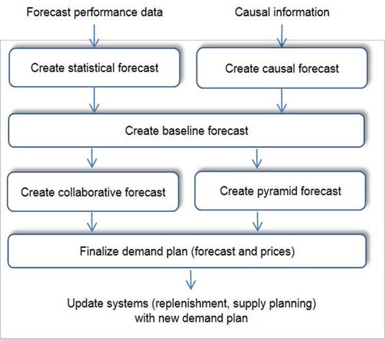
Figure 3-1. The demand planning process

Table 3-1. Relevance of Forecasting for Different Business Models

Business Model	Relevance
Make-to-order	Lead time for supply, assembly, and delivery is less than the lead time available to fulfill demand. No requirements for finished goods or raw material inventory. Not reliant on demand forecasts.
Assemble-to-order	Lead time for assembly and delivery is less than the lead time available to fulfill demand. Forecasting required to drive raw material inventory requirements.
Make-to-forecast	Lead time for assembly and deliver is greater than the lead time available to fulfill demand. Forecasting required to drive finished goods and raw material inventory.

Make-to-forecast, also termed make-to-stock, is characterized by a supply lead time that is greater than the customer lead time. This situation is very common for retail, distribution, and a majority of manufacturing businesses. The difference between the supply and customer lead time is a measure of the inventory exposure faced by the company. If the difference is large, then the company is required to take inventory positions well in advance of sales, resulting in greater exposure. For example, the customer lead time for a retailer is a few minutes (the time between a customer walking into the store and check-out), while the supply lead time is approximately four weeks. Similarly, an electronics manufacturer may be provided two weeks to fulfill a customer orders, but experience the same exposure due to a six-week supply lead time. Both these companies have to take an inventory position in order to provide a good customer experience.

Assemble-to-order is essentially a make-to-forecast system with the difference that final assembly can be postponed to occur after the order has been received from the customer. This postponed manufacturing step allows for several configurations to be supported with no finished goods inventory, and only raw material or sub-assembly inventory. If it is possible to re-design the product to convert from make-to-stock into assemble-to-order, this will result in lower inventory exposure.

The business model determines the processes and steps that need to be employed. For example, a make-to-order company will have less need for a forecasting process since material can be ordered after the customer’s order has been placed. Some examples of the relevance of the different processes for different business environments are shown in Table 3-2. As expected, manufacturers of make-to-stock products have the greatest need for the different demand planning processes.

Table 3-2. Use of Forecasting Methods by Industry

Tab2

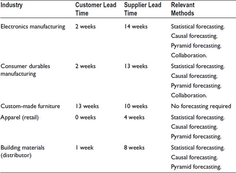
Each of these processes is described in the remaining sections of this chapter. Perusing them, you will appreciate that each of these processes has to be tailored to suit the unique requirements of each industry and company.

Measures of Forecast Performance

Forecast accuracy is the single most important metric for gauging the effectiveness of the forecasting process. Measures of accuracy include the following:

Forecast bias is a measure of constant under- or over-forecasting and is calculated as the average error per observation:

In Equation 3-1, d_i is the actual demand, d_i is the forecast for period i, and n is the number of periods. Under this definition, a positive bias indicates a trend toward under-forecasting, while a negative bias indicates over-forecasting.

The mean absolute deviation (MAD), a widely used measure of accuracy, is calculated as the average absolute error per observation,

Because MAD is calculated by summing absolute forecast errors, it is always greater than or equal to the bias.

Yet another measure is the root mean square error (RMSE), calculated as

RMSE is similar to MAD since it does not allow positive and negative errors across time to cancel each other (due to the square term). But the RMSE is different from MAD in that large variances have a greater influence on the measurement—mathematically, it has a standard deviation form. Therefore, RMSE is the appropriate measurement to be used in the safety-stock models (namely, the service level and newsvendor models) described in Chapter 2.

While MAD, bias, and RMSE measure the magnitude of error, a useful relative measure is the mean absolute percent error (MAPE), calculated as

MAPE is the most commonly used and most intuitive measure of forecast error.

Finally, forecast accuracy can be calculated from the MAPE as

Lagged Forecast Errors

For supply chains with extended lead times, it is not sufficient to monitor forecast accuracy for the same month (i.e., forecast for a month generated at the beginning of that month). The most widely used method for tracking 2- and 3-month-out forecast errors is the waterfall table, shown inFigure 3-2. This table is constructed by listing historical forecasts in rows, followed by the actual demand for each month. Then, forecast errors are calculated by comparing actual demand to the different forecasts for that month, as explained in the figure.

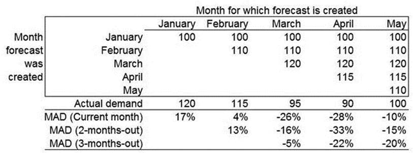
Figure 3-2. The waterfall table for calculating forecast errors

Explanation of the Lagged Forecast Error Calculations

March's current month forecast error
= (Actual for March - Forecast for March created in March) / Actual for March
= (95 - 120) / 95
= -26%.
March's 1-month-out forecast error
= (Actual for March - Forecast for March created in Feb) / Actual for March
= (95 - 110) / 95
= - 16%.
March's 2-months-out forecast error
= (Actual for March - Forecast for March created in Jan) / Actual for March
= (95 - 100) / 95
= -5%.

With this procedure, the forecaster can decide which measure of forecast accuracy needs to be utilized. If a product has a supply lead time of 3 weeks, then the current month error can be used to gauge forecast performance and for safety-stock calculations. However, if the supply lead time is 12 weeks, then the 2-month-out error needs to be used.

Demand Forecasting

The objective of the demand forecasting process is to specify an accurate estimate of the demand for the product into the future. Demand is affected by several factors, including:

· Established market. Market penetration and seasonal effects, reflected by historical demand data.

· Price. The occasional or regular change in price due to promotions can change demand significantly.

· Introduction of new products and entry into new markets. The company’s estimate of the market’s perception of a new product or in a new market may differ significantly from reality.

· The environment. Weather can magnify or shrink demand for certain goods, and it can impact several others by causing changes in the consumer’s buying patterns.

· Governmental policies. Hazardous material regulations, embargoes, and customs regulations are just a few factors that can change demand.

· Economic changes. Economic indicators reflect a change in the business environment that can foretell demand trends.

· Channel distortion. When a company sells its goods indirectly to the consumer through a sales channel, the biases introduced by the partner can significantly decrease forecast accuracy.

Each of these factors can be addressed by one or more methods, qualitative and quantitative. Qualitative methods consider subjective or personal experiences into the forecast. Some examples of qualitative methods are:

· Sales force forecasting. Individual forecasts from sales representatives and managers are added to arrive at the forecast. Because sales force forecasts frequently specify the financial projection for a product group, there is often a need for an additional translation step to convert this forecast into a unit forecast for a product.

· Delphi method. A panel of experts is asked their opinion of future demand. The experts are consulted separately in order to avoid the undue influence of a strong willed individual in a group setting. The experts could include executives in marketing and sales, as well as channel partners.

· Surveys. Consumer polls regarding responses to specific product features provide insight into market perception. This method is often used for new products.

Quantitative methods use statistical methods in order to arrive at a forecast. The most widely used quantitative methods are:

· Time series forecasting. A statistical method that uses historical demand data to calculate the forecast. This method assumes that all factors that impact demand are present in historical trends.

· Causal forecasting. This broadly refers to the consideration of factors that cause a change in demand, or lead demand in a determinable fashion. Examples include environmental, political, price, and economic factors. The most common mathematical method for creating causal forecast is regression.

Quantitative methods are less subject to bias than qualitative methods. (Bias is the consistent over- or under-prediction of demand.) However, qualitative methods are useful for incorporating information that is not reflected in the historical data but is known to the individual. As a result, a consensus method that utilizes both quantitative and qualitative forecast is used to reconcile differences. Examples of consensus methods are:

· Collaborative forecasting. This refers to the structured dialogues between retail and manufacturing partners. The objective of the collaboration is to communicate product demand, promotion, and expansion related information.

· Pyramid forecasting. This method refers to the entry of sales and managerial inputs at various levels in the product and geographic structure. These entries are reconciled with the numbers generated utilizing other methods, such as time series forecasts.

Most companies will find that a single forecasting method will not suffice, and there is a need to rely on several methods. The reason is due to the inherent difficulty in forecasting—predicting the future requires reliance on historical patterns, market conditions, competitive activity, environmental changes, and partner inputs. No one method addresses all of these different aspects. In fact, the accuracy of the forecast generated by each method can vary according to the forecast horizon (i.e., the number of months into the future for which the forecast is generated). Time series methods are usually accurate for shorter time horizons when new influences are not expected to affect product demand. Collaborative forecasting, which targets transparency between partners regarding advertising and promotion plans, is useful in the 2-to-6-month time frame because it provides visibility to new factors (for example, expansion into new markets). Causal forecasting, which can be used to generate forecasts based on environmental or economic conditions, is useful for both the short and long term since a variety of factors can be considered. Pyramid forecasting allows for the forecast from different organizations to be matched, and is an effective method for managing the entire forecasting horizon. Each of these methods is described in further detail in the following sections. Finally, a comparison of these methods is provided toward the end of the chapter.

Time Series Forecasting

Time series forecasting is a statistical method that uses historical sales data in order to estimate future sales. Time series models are ignorant about the causality that affects demand; instead, the models assume that all the causal effects are captured adequately in the historical sales data. Time series methods can be used to estimate level, trend, and seasonal effects. (A trend is a regular, slowly evolving change in the level of demand, whereas seasonality is a pattern that repeats after a time period.)

Moving Averages

The time series method that is most popular and easiest to employ is moving averages. In this method, the forecast for a particular product or product line is calculated by averaging the historical sales data over a specified number of periods. For example, a 3-month moving average would calculate the forecast as the average of sales for the last 3 months. This method results in a single value of forecast into the future. Therefore, moving averages ignores any trend and seasonality effects that are present in the data.

where n is the number of periods in the moving average, and t is the most recent period for which actual sales is available. An application of this method is illustrated in Example 3-1.

Single Exponential Smoothing

The moving averages forecast performed a simple average of past observations, with each observation being weighted equally. If the forecaster would like to give more weight to recent observations, an exponential smoothing model can be used. The simple form of exponential smoothing is also referred to as single exponential and the forecast is calculated as:

where α is the smoothing constant and has a value between 0 and 1.D_t is the actual demand for period t and F_t is the exponentially smoothed forecast for period t.

Larger values of α will give more weight to recent demands and utilize older demand data less than for smaller α. Therefore, large α will result in a more responsive and sometimes “nervous” forecast, while smaller α will produce a more stable forecast but will react slowly to changes in underlying demand.

Another way to write Equation 3-7 is to expand the forecast term F_t using the exponential smoothing formula. When this expansion is repeated for all forecast terms, the result is that the forecast can be calculated explicitly from historical sales data, as shown in Equation 3-8:

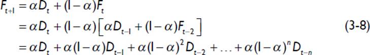
If the coefficients are plotted as shown in Figure 3-3, the higher weight placed on the most recent observation is easily seen, with the weight on earlier sales numbers being exponentially lower. For this reason, the method in Equation 3-8 is also referred to as exponential moving averages.

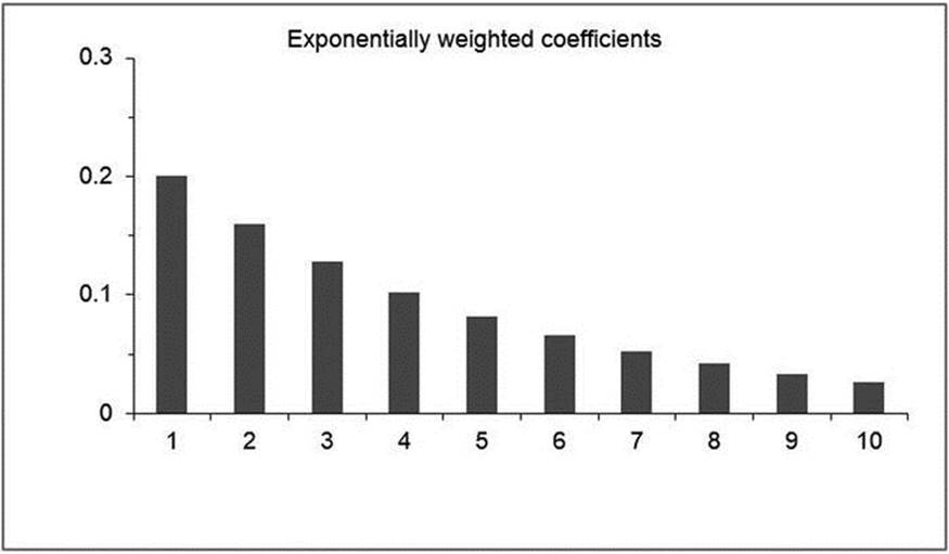
Figure 3-3. Weights applied to historical sales in the single exponential smoothing model (with α = 0.2)

While it easier to use Equation 3-7 for calculating forecasts, the form provided in Equation 3-8 is useful for understanding the nature of the calculation and why a higher value of α results in a greater weight on recent observations, while a lower value of α places a more uniform weight on recent and earlier observations.

EXAMPLE 3-1: FORECASTING USING TIME SERIES MODELS

The different methods are applied to the durable goods shipment data provided by the U.S. Census Bureau (specifically the UMDMVS series, where the U indicates seasonally unadjusted, MDM is the industry code for durable goods, and VS is the data code for value of shipments). The data is shown in Figure 3-4.

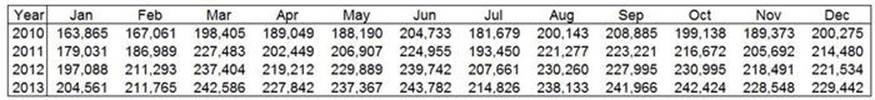
Figure 3-4. Durable goods shipment data ($ million) used in Example 3-1 (U.S. Census Bureau)

First, forecasts are generated using 6-month moving averages (MA) for years 2012 onward. The calculation is performed according to Equation 3-6, and the procedure is illustrated here:

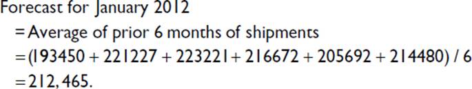
Because MA result in a stationary forecast (i.e., a single value for future periods), the forecast for February is the same as for January (212,465). As a result, the forecast errors are calculated as

The procedure is exceedingly simple, which is the reason that MA is so widely used.

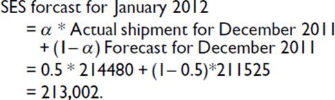
Next, forecasts are generated using single exponential smoothing (SES), with α = 0.5. Because this method uses the prior forecast, it requires a starting procedure to generate an initial value. This is achieved by setting the forecast for February 2010 equal to the actual shipment for January 2010—that is, 163,865. The March 2010 forecast is calculated according to Equation 3-7 as

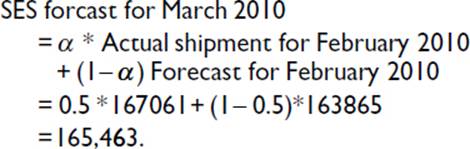
The procedure is repeated for subsequent months and results in a forecast for December 2011 of 211,525. With this value, the forecast for January 2012 is calculated as

Again, because SES results in a stationary forecast, the errors are calculated to be

Exponential smoothing is a more involved procedure than moving averages. The advantage of SES is that it naturally places a greater weight on the most recent observation. In addition, α is easily varied, which effectively increases or decreases the lookback period—a higher value of αdecreases the lookback period, whereas a lower value of α increases the lookback period.

Double Exponential Smoothing

The single exponential smoothing model results in a single value of forecast for the future (i.e., a stationary forecast). If there is a systematic pattern in the underlying data, then the model needs to be augmented to reflect the increasing or decreasing trend. The time series method that accounts for trends is called the trend-enhanced smoothed, double exponential smoothing, or Holt’s method. It involves two parameters (α for exponential smoothing and an additional parameter, β, for trend).

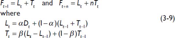
In Equation 3-9, L represents the level forecast, T represents the trend forecast, and D is actual demand. As with single exponential smoothing, starting values are required for initial level and trend estimates. One simple method is to set the level forecast as the first actual sales observation and the trend as the difference between the first two sales observations. Example 3-1 further illustrates the use of this method.

The data provided in Example 3-1, which are used to compute initial estimates for the level and trend forecasts, are obtained as follows:

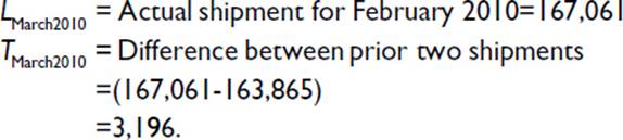
With these values, the forecast for March 2010 is calculated as

The forecast for April 2010 is calculated from Equation 3-9 as

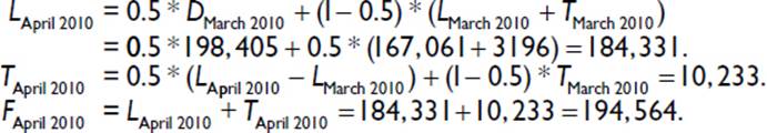
This procedure is repeated for subsequent periods, with the level and trend forecasts resulting in the following forecasts for January and February 2012:

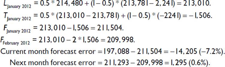
Unlike MA and SES, DES results in non-stationary forecasts. This is an important aspect because many businesses require forecasts to be generated for several months into the future so that operations can be appropriately planned. However, DES is not without its drawbacks. The first is that DES requires two parameters (Equation 3-9), which places an additional burden on the forecaster to determine the values to be used. Frequently, many forecasters simply set both parameters to 0.2. which results in a damped forecast. Once sufficient sales data has been gathered, the parameters can be determined from a trial-and-error procedure to determine values that minimize error.

The second drawback is related to the trend, inasmuch as the calculations for the third and subsequent periods are often too simplistic. In the example above, if an annual forecast is required, then the forecast for the 12th month would be . Examining prior sales data, it can be seen that this estimate is likely to be low. This simplistic approach is a problem experienced with DES for projections even two periods into the future. The business situations that require accounting for trends are usually for new products experiencing an initial ramp, obsoleting products experiencing a decrease in demand due to phase-out, or established products displaying a trend due to stronger or weaker adoption. The first two situations—new or obsolete products—are best dealt with in a manual fashion, with the ramp often being dictated by production capacity, or phase-outs being dictated by the timing of new product introductions. The third situation—established products displaying a trend—are often best dealt with using SES with a high value of α so that forecasts respond quickly to the underlying trend. Yet another method for dealing with this situation is to use pyramid forecasting to align product demand with revenue targets specified by management. This method is described later in this chapter.

Due to these drawbacks, the use of DES is often limited in practice. When it is used, it is often for just short-term forecasting (one or two periods).

Triple Exponential Smoothing

The methods described in the preceding section are adequate when the data displays a linear trend, but do not perform well when seasonality is present. Examples of seasonal trends are back-to-school for educational products, and Christmas for most consumer goods. A quarterly seasonal pattern is apparent in the durable goods shipments shown in Figure 3-5, with the third month of each calendar quarter displaying an uptick in demand.

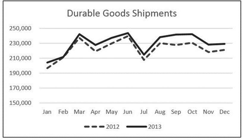
Figure 3-5. Seasonal patterns in durable goods shipment data ($ million) (U.S. Census Bureau)

The time series method that incorporates seasonality is referred to as triple exponential smoothing (TES) or the Holt-Winters method. It involves three parameters—the first parameter for level, the second for trend, and the third for seasonality.

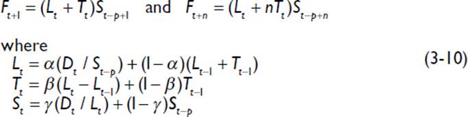
In Equation 3-10, S represents seasonal factors and p is the periodicity of demand. The procedure for implementing this method is illustrated below, using the data provided in Example 3-1.

The first step is to determine the periodicity of demand—the coefficient of auto-correlation can be used to determine this, and can be performed using a spreadsheet. The data for the first 2 years (i.e., 2010 and 2011) will be used to determine the period. If the shipment data is placed in a spreadsheet in cells A1 to A24, then the coefficient of correlation for a period of 2 months can be determined with the formula CORREL(A1:A22, A3:A24). Similarly, the coefficient of correlation for a period of 3 months can be determined with the formula CORREL(A1:A21, A4:A24). This calculation is repeated for various periods and the highest correlation coefficient indicates the period of demand. Performing the calculation for various combinations reveals that the coefficient of correlation is 0.57 for 3 month, 0.62 for 6 months, and has the highest value of 0.96 for 12 months. Therefore, the periodicity of demand is assumed to be 12 months.

The starting values for level and trend are the same as with DES; the starting values for the 12 seasonal indices are set to be 1.0. With this, the following initial forecasts are calculated for January 2012 as shown below.

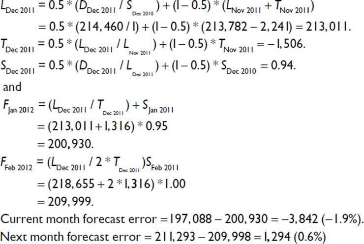
Note that, like DES, TES results in a non-stationary forecast, but this forecast has been further adjusted for a seasonal component based on the periodicity of demand.

The previous section discussed some of the drawbacks associated with trend-based forecasting. Because Equation 3-10 includes the same trend term, TES is subject to the same drawbacks; in fact, there is an additional parameter (γ) to be set, which increases complexity. However, an approach that is often used in practice is to generate a forecast considering only the level and seasonal term, so that the drawbacks to using a simplistic trend calculation for future periods are not an issue. This can be achieved by setting β = 0 in Equation 3-10 and setting the initial trend value to zero.

Because time series methods depend on sales history to discern patterns, any outliers can distort the demand picture and result in highly inaccurate forecasts. While it is enticing to remove outliers based on some statistical filter (such as any observation that is more than 2 standard deviations away from the 6-month moving average), this artificial modification of demand can have a detrimental effect on forecast accuracy if such deviations from the average can be expected in the future. It is far better to deal with outliers by understanding the nature of underlying demand signal and making adjustments accordingly, for example, by ignoring a special order from a customer undertaking a special one-time project. An example of this method is described in a later section on demand unawareness, which addresses non-recurring demand.

The methods and example demonstrated the use of historical data to create a forecast. These methods are effective when there is sufficient cause to believe that future demand will behave according to historical trends and patterns. However, there are several situations that do not lend themselves to history-based forecasting alone. Such situations include:

· Price-related influences, with future pricing trends being different from the past

· Expansion into new markets

· Weather impact, especially due to extreme weather situations

· Economic changes, such as changing interest and unemployment rates, and construction activity

· Distortion of demand when communicated by a channel partner, based on individual biases and ordering policies

These reasons result in a demand pattern that may deviate significantly from past history and therefore requires different forecasting approaches. Each of these issues is discussed in turn in the following sections.

Impact of Price on Demand

For most goods, a price drop will result in an increase in demand. When the quantity changes appreciably with price, the demand is termed elastic. In general, products that display elasticity have one or more of the following characteristics—they are not necessities, have substitutes, or are already priced low. On the other hand, necessities with no substitutes are inelastic and display little change in demand with price. The definition of price elasticity is

Price elasticity is negative for most products—i.e., a decrease in price results in an increase in demand, and an increase in price results in a decrease in demand. Additionally, when the absolute value of elasticity is greater than one, demand is considered to be elastic and a small change in price produces a relatively large change in demand. When the absolute value of elasticity is less than one, demand is considered to be inelastic and changes in price have little effect on demand volumes.

If data can be collected that clearly isolates the impact of price changes, elasticity can be determined easily. However, most demand data combines price changes with underlying trend and seasonal patterns, requiring that multiple factors be considered simultaneously. Regression methods can be used to understand the impact of price in isolation. Often, a simple model can provide the necessary insight, and allow for easy implementation of pricing related strategies. Example 3-2 exemplifies such a simple procedure.

EXAMPLE 3-2: FORECASTING THE EFFECT OF PRICE ON DEMAND

A manufacturer of lighting products measures its sales force on accuracy of revenue and units sold. Because regional sales managers have the authority to set price, the company wishes to provide them with price elasticity information so that revenue and volume analysis can be performed. How can this value be determined?

The forecaster uses a simple regression model of demand against price:

where d_i is the demand for period i, d_i-1 is the demand for period (i-1), p_i is the price for period i, and c₂ is the price elasticity. Such a model is applicable when the demand for a period is expected to be similar to the demand for the prior period.

The first step is to gather data related to historical sales and prices and perform the necessary calculations, as shown in Figure 3-6.

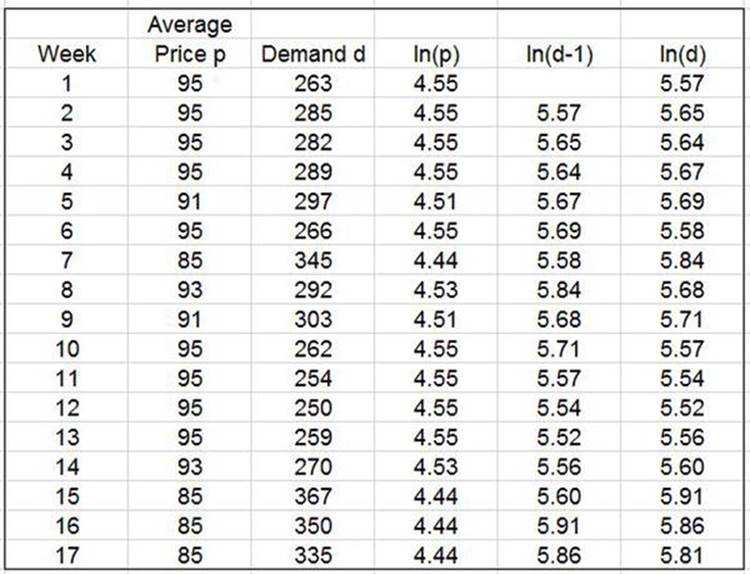
Figure 3-6. Regression model for determining impact of price on demand

Sales and price data has been collected for 17 weeks, and the final three columns are calculations based on this data. With the data arranged as shown, regression analysis can be performed using the spreadsheet function. The results are

The regression model reveals that the price elasticity is -2.32, with a coefficient of determination of 0.87. Because the absolute value of elasticity is greater than 1, this indicates that the product experiences elastic demand and is sensitive to price changes. From this equation, the sales managers can use the simple rule that a 1% decrease in price will result in a 2.3% increase in demand volumes.

There are several challenges faced when trying to incorporate price. First, assuming that demand is dependent only on price may not be accurate since other factors can contribute to fluctuations (such as weather and seasonality). Therefore, in order for the price model to provide an accurate relationship, it is necessary to select a duration over which the impact is known to be primarily price, or to increase the complexity of the model to include other affecting factors. Second, price changes can impact demand in the same period, as well as subsequent periods. Price reductions provide an incentive for the consumer to purchase goods earlier than planned, resulting in a shift of demand to the current period. In such cases, additional price terms need to be included in the model. Finally, elasticity depends on demographic factors such as age and income, as well as store level considerations such as competing items and retailers. The model developed in the example provides no insight into the fundamental nature of elasticity. Detailed models can provide the fundamental insights, but have significantly greater data requirements related to daily sales, promotions, and in-store coupon information, data for competing products, and the proximity of competing stores.¹

Market Expansion

New product forecasting requires that sales estimates be made by considering several factors, including market size, product characteristics, time required for adoption, price points, and competitive products. Since the impact of each of these factors is uncertain, forecasting the demand for new products is a challenging task. Some of the methods used are:

· Market analysis. Such a method starts with an estimate of the total market potential, and then reductions are made to this number according to product features, price, and competitive factors.

· Analogous forecasting. This popular method maps the sales profile or an existing, similar product to the new product. While seasonal and lifecycle profiles are retained, lifecycle or annual volumes can be modified based on a market analysis for the new product.

· Diffusion modeling. The adoption of a product is perceived to go through the following steps: Awareness, interest, evaluation, trial, and adoption. The diffusion model uses an S-shaped curve that models several of these aspects and forecasts sales over time.²

On the other hand, market expansion refers to the introduction of existing products into new geographies and stores. Since the product is not new, sales numbers from existing markets are available, providing valuable information regarding market size and consumer perceptions. Diffusion effects, while present, can be significantly accelerated due to the awareness that has already been created in the marketplace. As with new products, sales estimates for new markets can be estimated in a few different ways: One method is to use guidance provided by channel partners or judgmental methods. Yet another is to derive a forecast based on sales for another product being sold in that market; the accuracy of such a forecast depends on how similar the products are.

When channel guidance and similar-product sales are not reliable, demographic analysis is an alternative for arriving at a forecast. The effect of demographics on sales differs by industry. For example, an annual report of Bausch & Lomb, a manufacturer of eye health products, identifies age as an important demographic:

We expect drivers of sales and earnings growth over the next several years to include:

· A continued focus on faster growing business segments and the launch of higher-margin new products in each of our product categories;

· Favorable demographic trends, such as the aging of the population and an increase in the incidence of myopia and presbyopia; and

· Opportunities to further implement lean manufacturing techniques and other cost improvements to enhance margins, particularly for contact lenses and intraocular lenses.

—Bausch & Lomb, Inc., 2007 Annual Report

Similarly, an annual report of the Dr. Pepper Snapple Group, a beverage manufacturer, identifies a different set of demographics:

We are impacted by shifting consumer demographics and needs. We believe marketing and product innovations that target fast growing population segments, such as the Hispanic community in the U.S., could drive market growth. Additionally, as more consumers are faced with a busy and on-the-go lifestyle, sales of single-serve beverages could increase, which typically have higher margins.

—Dr. Pepper Snapple Group, 2013 Annual Report

An annual report of Sonic Corporation, a restaurant chain, identifies additional demographic factors:

Franchise Drive-In Development. We assist each franchisee in selecting sites and developing Sonic Drive-Ins. Each franchisee has responsibility for selecting the franchisee’s drive-in location but must obtain our approval of each Sonic Drive-In design and each location based on accessibility and visibility of the site and targeted demographic factors, including population density, income, age, and traffic. We provide our franchisees with the physical specifications for the typical Sonic Drive-In.

—Sonic Corp., 2009 Annual Report

Clearly, the characteristics of the product determine the specific demographic factors that need to be considered. Some of the most common factors are:

· Population. Often a starting point in estimating market opportunity, population-based estimates may not yield good results for products that appeal to only a particular section of the population. As a result, additional factors, such as age or education, are often considered in addition to population.

· Age. Segmentation of age provides visibility to market opportunity for products for specific ages. Additionally, age has been found to be a factor in responsiveness to price changes, with elderly people being more sensitive to price in general.

· Ethnicity. Provides visibility to market opportunity for products geared toward specific ethnic populations.

· Educational attainment. College education is often an indicator of market opportunity for products that require research or are geared toward specialists. This could include health foods as well as high-end electronic items.

· Income. An important factor in determining market opportunity, income also plays a role in determining price sensitivity. Higher income is often equated with low elasticity, reducing the effect of price reductions. Indeed, there are cases when higher income can result in positive values for elasticity (reference 8).

· Household size. An important indicator of market opportunity, household size also factors into responsiveness to price changes. Larger households are more sensitive to price changes (reference 9).

· Housing units. The number of housing structures, as well as the number of units in each structure, is a useful indicator for several class of building materials.

Demographic analysis can be performed according to the following steps. First, demand data is collected for several different geographies. Usually, quarterly or annual data is used so that demand is not skewed by timing of sales or seasonality that can arise from weekly or monthly data. The second step is to identify demographic variables that have the capability of influencing sales and to collect this data for the identified geographies. The third step is to construct a regression model and generate results. Any adjustments to the variables are made until an acceptable correlation has been identified. Finally, the resulting forecast can be converted into monthly numbers by applying appropriate seasonal variables from existing markets, as well as ramp-up modifications to capture diffusion effects related to awareness. These steps are illustrated in Example 3-3.

EXAMPLE 3-3: NEW MARKET FORECASTING

The following annual sales data is available for a home remodeling product for eight metropolitan areas in the United States.

Region	Annual Sales ($ Million)
Atlanta, Georgia	3.9
Boston, Massachusetts	7.6
Minneapolis, Minnesota	3.2
Norfolk, Virginia	1.1
Philadelphia, Pennsylvania	16.0
St. Louis, Missouri	2.1
Washington, D.C.	11.5

Since the remodeling product provides additional structural space in the house, the forecaster believes that two factors that contribute to sales are housing units and household income. In particular, attached units in 1-4 unit structures, with tight space constraints, are the main target, and the relevant data is shown in the following table.

Region	Number of 1-4 Household Units	Household Income (Median)³
Atlanta	152,599	51,948
Boston	406,506	55,234
Minneapolis	155,086	54,370
Norfolk	118,078	42,472
Philadelphia	743,689	45,862
St. Louis	129,446	43,432
Washington, D.C.	362,226	70,206

With this data, it is possible for the forecaster to perform a log-linear regression analysis of sales versus the demographic variables. The results of the analysis are shown in Figure 3-7.

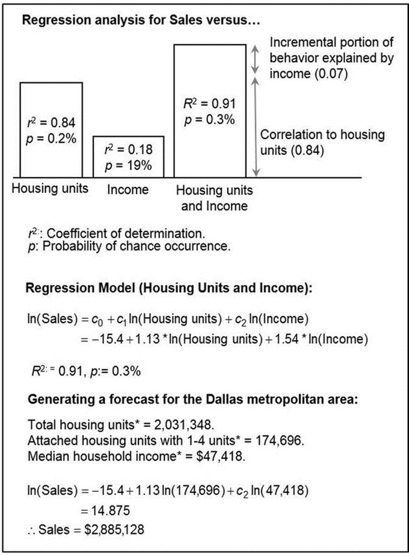
Figure 3-7. Forecasting using demographic data

The results indicate that the sales numbers have a strong correlation with housing units, and secondarily with income. Given the strong correlation from the combined model, it can be used for estimating sales for the new market. An example of the procedure for generating a sales forecast for the Dallas (Texas) metropolitan area are also shown.

Example 3-3 demonstrated the use of demographic information for the home remodeling industry. Products in other industries may be influenced by different demographic factors. The guidelines provided in Table 3-3 may be used as a starting point for analysis.

Table 3-3. Examples of Relevance of Demographic Data by Industry

Industry	Relevant Demographics
Apparel, consumer goods (non-durables)	Population, age, ethnicity, household income.
Consumer goods (durables)	Housing units, duration of occupancy, household income.
Building materials	Housing units, age and value of house, household income.
Consumer electronics	Population, education, household income.

In conclusion, demographic analysis can be useful for understanding the business potential of new markets. The wealth of demographic information collected in most countries allows for the construction of insightful regression models.

Weather Impact

Weather can have a significant impact on sales of products and services in several industries. Consider the following statement from Lennox International, a manufacturer of air conditioning and heating equipment:

Demand for our products and for our services is seasonal and strongly affected by the weather. Cooler than normal summers depress our sales of replacement air conditioning and refrigeration products and services. Similarly, warmer than normal winters have the same effect on our heating products and services

—Lennox International, Inc., 2013 Annual Report

Such an impact is common for building material manufacturers. In addition, retail industry sales are also influenced by weather due to the impact of extreme weather conditions on consumer traffic. An insightful study into this subject has been provided in the paper, “The Effects of Weather on Retail Sales” by Martha Starr-McCluer.⁴ The method and findings of this paper are summarized as follows:

· Consumer spending is captured using monthly retail sales data from the U.S. Census Bureau, based on a survey of about 12,000 retail establishments.

· Weather data is captured using degree day data from the National Weather Service. According to this convention, a heating degree day occurs if the average temperature for a day exceeds 65 degrees Fahrenheit, and a cooling degree day occurs if the average temperature is below 65 degrees Fahrenheit. For the entire United States, monthly heating and cooling degree days are computed as the population-weighted averages of degree days at the individual weather stations. Since the study focuses on temperatures that depart from seasonal norms, the degree days for a particular year are compared against the seven-year average.

· The correlation between weather and retail sales is studied using a regression model. The model takes several factors into account, including degree-day variances for four periods to account for lagged effects, real labor income, stock prices, and interest rates.

· The results indicate that unusual weather has a modest but significant role in explaining monthly sales fluctuations. The incremental R-square (coefficient of determination) is 9.7%, which is a measure of the level that weather impacted retail sales. As can be expected, the incremental R-square was highest for building materials (18.4%), general merchandise (21.3%), and restaurants (13.9%).

If the effects are significant at a macro-economic level, what about for individual companies? A logical argument would indicate that the effects should increase, due to substitution. At the product level, increase in consumer activity could result in an increased demand for a particular product. If that product is not in inventory, the consumer may settle for a substitutable product. In such cases, product and company sales are affected, even though aggregate sales are not.

While the paper describes a method for incorporating weather effects at an aggregate level (across broad product categories and geographies), developing models for specific products and locations requires a different approach that incorporates, in addition, recent sales history and location-specific effects. For a broad category of products and services, a common effect of weather is to modify demand patterns. Consider the construction industry: An unusually warm winter can result in an early start for new house construction. An increase in the total units built for the year is not guaranteed, but the early start creates requirements for building material to be available earlier than usual.

Similarly, an early spring can result in early demand for spring clothing. If the retailer’s inventory is largely winter clothing, there is a high probability of losing sales to competitors, with limited chance for recovery.

On an operational level, severe weather can cause certain purchases to be made earlier and stockpiled, for example, groceries. If the retailer is unprepared, this can result in stockout situations for products such as milk, bread, and other food items.

For another category of products, weather can have a causal impact on demand, resulting in new demand that would otherwise not be present. A few popular examples include the effect of unusually cold temperatures on demand for new heaters and car batteries, and the impact of unusually warm temperatures on air conditioners. Several grocery items show similar trends, examples include ice creams, soups, and beverages. Apart from physical goods, the service industry is also impacted, for example repair services for air conditioners, heaters, cars, and telecommunication equipment.

A simple weather model that relates demand to temperatures is expressed as

In Equation 3-12, i is the time period and ΔT is the difference in observed temperature for period i from historical averages. Such a model can be used to estimate sales of products that are influenced by weather, such as air conditioners.

However, it might not be possible to get the desired level of accuracy from such a simple model. Challenges complicating the construction of detailed weather models include the following:

· Multiple weather variables. Weather can affect sales in many ways, by a combination of precipitation, temperature, wind, and extreme weather. The model needs to include all these variables and interactions.

· Complex weather patterns. Weather effects can persist across daily and weekly periods, increasing the number of interactions and complexity.

· Large data volumes. Data requirements are significant, with data having to be collected for each city or geography, along with historical averages. An additional complication arises when demand is for a geography that covers several cities. In this case, weather variables are to be calculated as the population-averaged temperature across all the cities. When a company has several hundreds or even thousands of products, it is quite an undertaking to build and maintain these models.

· Underlying inaccuracy in weather forecast. Yet another drawback with weather models is that predictions are made based on the weather forecast, which itself is subject to error. Due to this inherent lack of accuracy, even sophisticated models that consider several weather factors may not deliver the anticipated improvement in accuracy.

While these challenges are obstacles, there are still ways to use weather for operational improvements. The model can be converted into simple rules that can provide a good balance between complexity and ease of use. For example, consider the guideline for demand for air conditioners: “Sales of entry-level air conditioners increase by 2% for every one-degree Fahrenheit increase in temperature above normal.” Such a guideline can easily be used to modify forecasts, because data requirements are minimal and can be collected easily.

When severe weather has the effect of shifting demand patterns, daily operational adjustments can be made without reliance on sophisticated mathematical models. Instead, making a simple adjustment to the forecast that increases demand levels prior to a storm, and decreases it during the storm will result in a better positioning of inventory. For example, consider demand for certain grocery items. While smaller storms may have little impact on purchasing patterns, snowstorms that pose the threat of inhibiting consumer mobility will alter buying patterns and result in milk purchases being made earlier.

In conclusion, weather can have a significant impact on demand for products for which precipitation and temperature have a causal effect. For other products, weather mainly has the impact of shifting the timing of demand, which can be addressed using safety stock. Extreme weather conditions will require special attention since inventory buffers may be insufficient.

Economic Indicators

Theoretically, almost every company can benefit by considering one or more economic indicators of market conditions into the forecasting process. These indicators include, for example, retail sales and inventories, manufacturer shipment and inventories, unemployment, housing permits, and the consumer price index. The following excerpt from an annual report of a construction materials manufacturer provides an indication of how market conditions can impact a business:

For the new residential construction market, housing starts are a very good indicator of demand for our gypsum products. Installation of our gypsum products typically follows the start of construction by one to two months.

Demand for our products from new nonresidential construction is determined by floor space for which contracts are signed. Installation of gypsum and ceilings products typically follows signing of construction contracts by about 12 to 18 months. According to McGraw-Hill Construction’s most recent construction market forecast, total floor space for which new nonresidential construction contracts were signed in the United States increased 5% in 2013 compared with 2012.

The repair and remodel market includes renovation of both residential and nonresidential buildings. The generally rising levels of existing home sales and home resale values in 2012, and continuing into 2013, have contributed to an increase in demand for our products from the residential repair and remodel market in 2013.

—United States Gypsum Corporation, 2013 Annual Report

The report indicates that various indicators of construction activity can be used to adjust forecasts and improve accuracy. The use of such data for long-term projections of market size is well addressed. However, the utility of such data to short-term, product-level forecasting is constrained by the following considerations:

· Industry categories are too broad. Several of the indicators are specified at the national level, or for an industry that encompasses several categories of products. As a result, it is not clear how to translate a change in the economic variable into a change in demand for a specific product and geography. For example, retail sales for electronic items may trend up in a particular month, but the implications of this change for trendy music players may be very different from staid alarm clocks.

· Delay in disseminating data. Most indicators are collected based on polls and surveys of businesses. The delay due to data collection and dissemination to the public makes some of the information useless for forecasting purposes. For example, a forecaster for a manufacturing company will have little to gain from a report that states that two-month prior retail sales have decreased, since the company’s backlog would already reflect that trend.

To use economic indicators effectively, a company needs to follow a procedure for identifying indicators that are important to the business and capable of providing insight, given the timing of its updates. The properties of a selection of such indicators are shown in Table 3-4.

Table 3-4. Selected Economic Indicators for a Building Material

Tab4

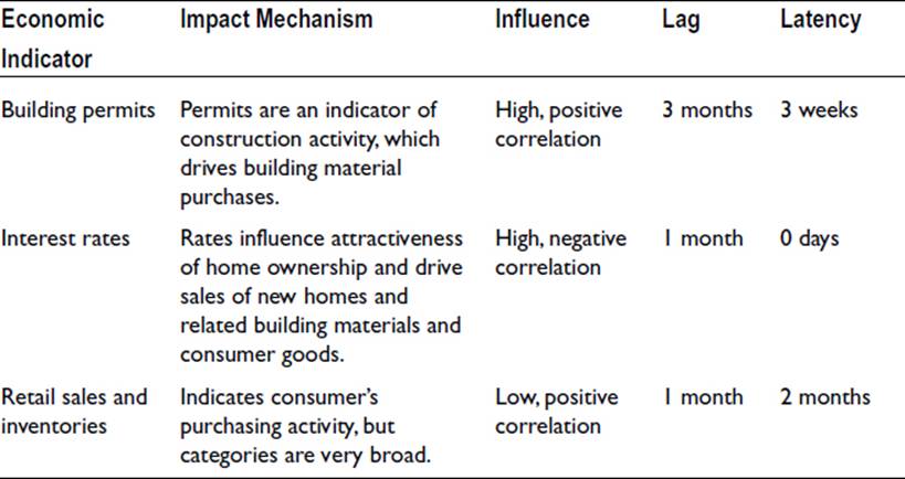
Table 3-4 characterizes indicators in a descriptive manner, but it is possible for the relationship to be expressed quantitatively using regression. The lag is the time it takes to impact demand after the indicator has changed. For example, if an increase in building permits in a particular month results in an increase in demand three months later, the lag is three months. Latency refers to the time taken to report data. Because building permit data in the United States is released by the U.S. Census Bureau in the third week of a month for the prior month, the latency is three weeks. If the latency is greater than the lag, the economic indicator provides no new information that the company is not already aware of. From the table, building permits and interest rates provide information that allows the company sufficient time to adjust supply levels according to demand, while retail sales provide no benefit due to the high latency present in collecting and disseminating the data.

The two indicators, building permits and interest rates, are both plausibly suggestive, but it is necessary to ensure that there is no interdependence between them. Because interest rates can affect applications for building permits, it may not be necessary or accurate to include both in the forecasting process. Instead, permits alone can be used because the information is provided at the detailed city-level, allowing for greater accuracy in evaluating the impact of interest rates on different regions and capturing pockets of development.

The list of pertinent indicators can look different for other products in the same industry. For example, the insight provided by building permits will be less useful for concrete due to the one month lag between permitting and the demand for concrete. Clearly, the larger the difference between the lag and the latency, the more useful the indicator.

To understand how economic indicators can be used in forecasting, quarterly revenue numbers from some publicly traded companies may be fit to quarterly building permit data using Equation 3-13:

In Equation 3-13, t is time, k is the lag in quarters, and P_t-k is the lagged building permits. If k is equal to 0, then there is no lag at a quarterly level. If k = 1, then there is a lag of a quarter. An application of this model is demonstrated in Example 3-4, with revenues for selected public companies being related to building permits.

EXAMPLE 3-4: IMPACT OF ECONOMIC ACTIVITY ON REVENUES

In this example, revenue data from public companies is used to evaluate the impact of leading economic indicators. In general, such an analysis will not yield good results due to the many nuances that influence reported revenues, such as revenue recognition, quarterly data, accounting rules, and product diversification. However, this example serves the useful purpose of clarifying how a model can be constructed using the identified indicators.

The significance of housing activity on four companies is studied—Lennox International, Weyerhaeuser, Pittsburgh Paints, and Best Buy. Lennox is a manufacturer of air conditioners and sells to the home builders as well as to retail channels. Weyerhaeuser manufactures lumber products for homebuilders and retail channels. Pittsburgh Paints is a large paint manufacturer, again with a diversified customer base. Finally, Best Buy is an electronics retailer. The reason for including Best Buy in the study to test the hypothesis that purchases of big ticket electronic items are linked to purchases of new homes.

For each of the companies, 15 quarters of revenue data is collected from the respective annual reports (from Q1 2003 until Q3 2006) and permit data is obtained from the U.S. Census Bureau. An example of this data for one of the companies, Lennox, is shown in Table 3-5.

Table 3-5. Lennox Revenue and Housing Permit Data⁵

Quarter	Revenues ($ Million)	Permits Issued
Q4 2002		388,275
Q1 2003	$586	371,662
Q2 2003	$746	463,520
Q3 2003	$758	464,434
Q4 2003	$700	422,893
Q1 2004	$664	430,673
Q2 2004	$805	538,632
Q3 2004	$772	510,181
Q4 2004	$741	457,956
Q1 2005	$700	441,907
Q2 2005	$868	537,059
Q3 2005	$928	527,929
Q4 2005	$841	443,388
Q1 2006	$800	461,834
Q2 2006	$1,002	484,221
Q3 2006	$1,007	396,402

The results of applying the regression model are summarized in Figure 3-8.

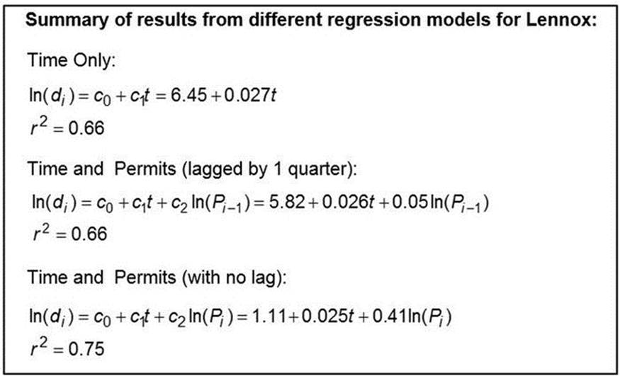
Figure 3-8. Results from forecasts using economic indicators (Example 3-4)

The results reveal that the inclusion of permits from the current quarter has been successful in explaining an additional 9% of revenue behavior as compared to the model that ignores the effect of permits. On the other hand, inclusion of permits lagged by one quarter has no effect on the results, indicating that the products manufactured by Lennox are sold to home builders within 3 months of permitting. A similar analysis is performed for the remaining companies and the results are summarized in Table 3-6.

Table 3-6. Summary of Results of Forecasts Using Building Permits

Tab6

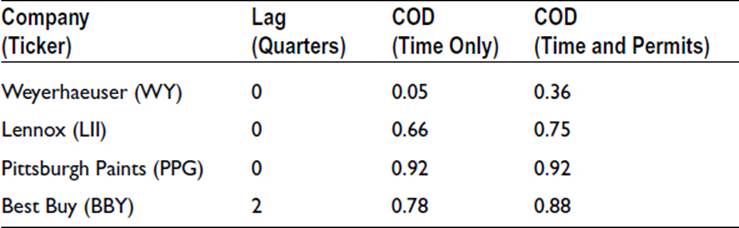
The results are mixed. As expected, including permit data improves model performance] for Weyerhaeuser and Lennox, although the remaining unexplained variance for Weyerhaeuser is large. The results for Pittsburgh Paints indicate that the proportion of the company’s business attributed to construction activity is minimal. The results from Best Buy are interesting and support the hypothesis that purchases of large ticket electronic items are linked to new home sales, approximately 6 months after permitting.

This example reveals that certain insight into demand may be obtained by utilizing construction data. The use of quarterly numbers reduces the value from the model since a zero lag provides no advance visibility. However, use of monthly product sales and construction data may address this issue.

In conclusion, economic indicators are very useful in capturing nationwide trends in business. However, demand for a product can be heavily influenced by local trends that are contrary to macroeconomic indicators. Therefore, when available, micro-economic data is useful for generating detailed product forecasts.

Distortion of Demand Information

When a company sells directly to the consumer, it is possible to get a first-hand view of demand. However, when a company sells its products to manufacturers and distribution partners, the partner’s demand signal is often used as a proxy for consumer demand. A few of the challenges related to indirect sales are captured in an annual report of Hewlett-Packard:

We must manage inventory effectively, particularly with respect to sales to distributors, which involves forecasting demand and pricing issues. Distributors may increase orders during periods of product shortages, cancel orders if their inventory is too high or delay orders in anticipation of new products. Distributors also may adjust their orders in response to the supply of our products and the products of our competitors and seasonal fluctuations in end-user demand. Our reliance upon indirect distribution methods may reduce visibility to demand and pricing issues, and therefore make forecasting more difficult. If we have excess or obsolete inventory, we may have to reduce our prices and write down inventory. Moreover, our use of indirect distribution channels may limit our willingness or ability to adjust prices quickly and otherwise to respond to pricing changes by competitors. We also may have limited ability to estimate future product rebate redemptions in order to price our products effectively.

—Hewlett-Packard Company, 2007 Annual Report

A phenomenon, often referred to as the bullwhip effect, states that demand information is distorted as it is communicated by partners.⁶ Distortion does not occur due to willful actions on part of the partner, but due to each entity attempting to deal with the observed demand in isolation. Some of the common reasons for distortion are a lack of awareness of the composition of demand, multiple forecast updates, and replenishment and ordering policies. This distortion is illustrated in Examples 3-5 and 3-6, which are followed by a detailed discussion of the reasons.

EXAMPLE 3-5: INFORMATION DISTORTION DUE TO A PULSE DEMAND SIGNAL

Consider the situation of a retail sourcing goods from a manufacturer. In turn, the manufacturer purchases raw material from a supplier. The retailer’s demand for the product is a steady 100 units per week, except for a particular week when a promotion has increased the sales by 10 units. The demand reverts to 100 units for subsequent weeks. Furthermore, the retailer is supplied immediately by the manufacturer (i.e., a zero lead time), the manufacturer has a 1-week lead time for parts, and the supplier has a 2-week lead time for raw material.

First, the manufacturer’s inventory positions are examined: Since the manufacturer has planned for a steady demand for 100 units, the increase by 10 units will reduce inventory positions and require additional supplies. Also, the manufacturer calculates a demand forecast based on a 2-week moving average of the retailer’s orders. This results in a forecast for the next week of 105 units. Given the 1-week lead time for part supply, the order placed by the manufacturer is calculated as

Part order = Cycle stock + Safety stock = 105 + 10 = 115 units.

Next, the part supplier’s inventory positions are examined. The increase in demand as seen by the supplier is 15 units, which depletes safety stock by the same level. The supplier calculates a demand forecast based on a 2-week moving average of the manufacturer’s orders, which results in a forecast for raw material of 108 units. Given the 2-week lead time for part supply, the order placed by the manufacturer is calculated as:

Raw material order = Cycle stock + Safety stock = 108 + 15 = 123 units.

The propagation of the demand signal across the stages in the supply chain is shown in Figure 3-9.

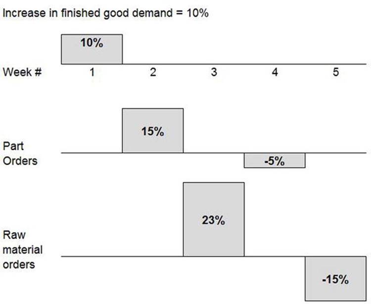
Figure 3-9. Distortion of information due to the demand pulse in Example 3-5

A few observations can be made from the results. The first is that the initial fluctuations of orders for the part and raw material are larger than the increase in demand. In order to compensate for these additional units ordered, there is a decrease in the order quantity in subsequent periods. The magnitude and duration of fluctuations increase as the signal propagates further along the supply chain.

The second observation is that the extent of distortion is affected by lead times. The lead times in the example were set to 1 week for the part and 2 weeks for the raw material. If these are increased to 2 and 4 weeks, respectively, the associated magnitude of distortion is significantly different. The part order increases from 15% to 20%, while the raw material order increases from 23% to 39%. The difference is due to the accumulation of forecast errors over the lead time. Therefore, the adverse impact of distortion increases with increasing lead times.

The example uses two-period moving averages to compute the forecast, which results in a forecast that is very responsive to new trends and increases the magnitude of distortion. It is enticing to think that the use of four- or eight-period moving averages or other such methods can reduce the magnitude of the fluctuations. However, an increase in damping introduces distortion when the change in demand is sustained, as illustrated in Example 3-6.

EXAMPLE 3-6: INFORMATION DISTORTION DUE TO SUSTAINED CHANGE IN DEMAND

The supply chain is identical to Example 3-5, except that the retailer experiences a permanent increase from 100 to 110 units per week due to the opening of a new store. Additionally, the manufacturer and supplier generate forecasts using 4-week moving averages (as opposed to the 2-week moving averages used in the previous example).

The manufacturer’s and supplier’s inventory positions are examined according to the procedure described in the previous example, and the resulting signals are shown in Figure 3-10.

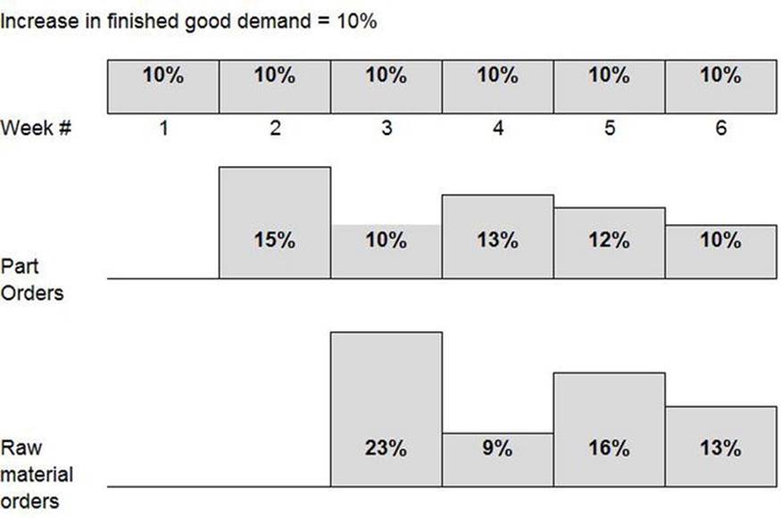
Figure 3-10. Distortion of information due to a demand pulse (Example 3-6)

Since the demand increase is sustained, the orders fluctuate and gradually settle at a level equal to the increased demand. While the magnitude of the fluctuations are lower due to the use of 4-week moving averages, additional time is required to reach steady state. Indeed, if 8-week moving averages are used, the fluctuations would continue for several additional periods.

In conclusion, information distortion cannot be solved using a highly damped or a responsive forecasting method. Instead, it is necessary to understand the sources of distortion and deal with them accordingly. Some common causes of distortion are discussed in the following sections.

Demand Unawareness

The total demand number is actually a combination of several underlying sources and mechanisms, such as retail store sales and contract sales to businesses. Distortion can occur when a single forecasting method is applied to all categories indiscriminately. For example, a large one-time sale will result in a pulse demand signal. Time series methods should not be used for this category of demand.

For the purposes of understanding distortion, demand may be divided into two categories—recurring and nonrecurring. Recurring demand refers to the portion of demand that is captured adequately by historical data and is expected to repeat over time, such as sales of an established product at an existing store. Time series forecasting methods are well suited for dealing with recurring demand.

Nonrecurring demand includes sources and causes that are not expected to repeat in the near future. This includes special contract sales (such as one-time sales to large customers), initial stock at a new facility, and one-time purchases for store displays. Since this category of demand is not expected to recur in the near future, the nonrecurring volume needs to be removed from overall demand numbers before applying a time series method. A pulse signal, illustrated in Example 3-5, is an example of nonrecurring demand.

Promotions can increase demand temporarily and surprise the uninformed manufacturer. Promotional demand is nonrecurring and needs to be flagged accordingly. However, inventory planning may need to be performed differently for promotions if the increase in demand is accompanied by a brief lull following the promotion.

The lack of awareness of demand sources is not restricted to interactions between companies, but can exist even within a company. For example, it is quite common for marketing to communicate only an aggregate demand number to the supply chain analyst, without any additional details regarding sources or categories or demand. While communications in a company can be improved relatively easily by requiring a dialogue between marketing and SCM as part of the forecasting process, it is a bigger issue when multiple companies are involved. In order for retailers, distributors, and manufacturers to improve demand visibility, a structured collaborative forecasting process is required.

The importance of segmenting non-recurring demand is illustrated in Figure 3-11, where data for weeks 2 and 3 have been skewed by one-time orders. If forecasts are generated using 6-week moving averages, the difference in forecasts generated based on total demand as compared to only recurring demand can be significant.

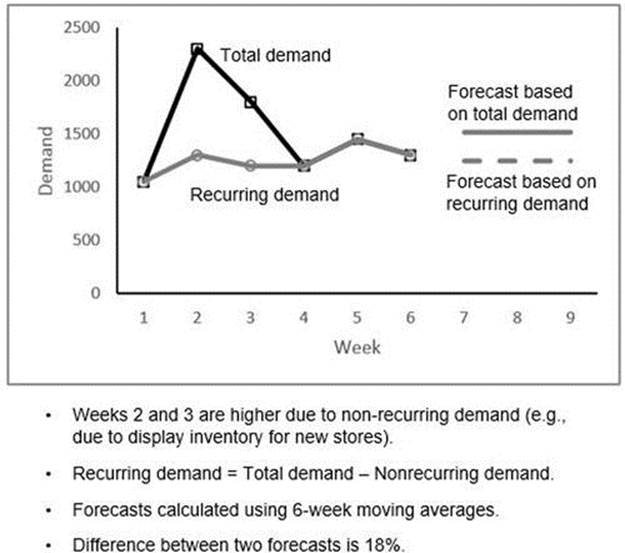
Figure 3-11. The importance of segmenting nonrecurring demand in forecasting

Multiple Forecast Updates

An increase in the number of entities involved in generating or modifying the forecast is often accompanied by an increase in the bias, and eventually, distortions. If a manufacturer has access to actual sales or point-of-sale (POS) data, the manufacturer’s forecast can be generated by applying appropriate methods (for example, time series). Some of the advantages of using POS data are:

· Good visibility. POS data provides a view of actual consumer demand, undistorted by biases and ordering policies utilized by the retailer.

· Frequent updates. The regular communication of orders and forecasts provide manufacturers with visibility to trends only on a weekly or monthly basis. POS data provides the manufacturer immediate visibility to changes and allows actions to be taken several days or weeks in advance.

The fine-grained demand information provided by POS data can provide valuable insights regarding buying trends, and can be used to plan promotions and placement of inventory by region or by the days of the week. Furthermore, availability of POS data can lead to vendor-managed inventory (VMI), with the supplier being given the responsibility of maintaining the targeted inventory and customer service levels. However, there are challenges in using POS data, such as:

· High data volumes. Since POS information is collected at a store level, this often results in extremely large volumes of data.

· Lead time mismatches. If the manufacturer replenishes the retailer’s distribution center, then there is a time lag between sales data and replenishments. Therefore, the analyst needs to explicitly account for these time lags before acting on POS data.

· Lack of context. POS data can be misleading due to incomplete information. For example, no sales for a day could be due to a lack of movement of the product, or due to a stockout situation. If it is due to the latter, a forecast generated using time series methods can result in misalignment between the demand and supply.

The first issue requires that the manufacturer deploy a system that can collect and process the data to ensure speedy processing and aggregation. Such a system is critical for continued use of POS data, since it can help deal with operational issues such as a store not reporting sales, or the addition of new stores.

The second issue related to misleading data needs to be addressed by understanding the nature of the issue. Consider the issue related to no sales being reported at a particular store for the duration of a day or more (see Figure 3-12). This situation can arise due to a malfunctioning POS system or due to an out-of-stock (OOS) situation. In both cases, the POS data does not reflect the true demand. In such cases, the POS data needs to be adjusted to reflect missed demand for those days; for example, the prior 8-week average sales can be used.

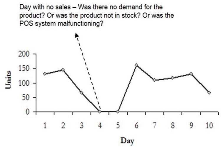
Figure 3-12. Sample point-of-sales (POS) data for a store

However, if there are consistently days with no sales, this could be due to poor inventory management or due to sporadic demand for the product. For the former, adjusting POS data to fill in low-sale days will improve results. For the latter, adjusting sales will only increase shelf inventory without additional sales. Therefore, it is important to determine the reason for low values. Often, the forecaster can provide the necessary insight from experience and an understanding of the retail situation. Alternatively, the cause can be determined by studying inventory levels in the store to determine if sufficient stock existed. If the manufacturer ships its goods directly to the store (direct-store delivery), this inventory information will be readily available. Otherwise, if the store is a high revenue generator, merchandising personnel can perform the store visit.

Finally, POS data alone cannot provide all the information required to estimate future demand. Since demand is affected by promotions and price, as well as the introduction of new markets or additional units for display purposes, POS data needs to be augmented with collaborative forecasting to capture any additional information.

In conclusion, point-of-sale data can provide valuable insights and reduce out-of-stock situations. However, challenges related to the volume and quality of data need to be addressed before the information can be used with confidence.

Ordering and Replenishment Policies

Distortion can also be introduced due to improper inventory management and replenishment processes on the part of the channel partner. Some examples of channel partner actions that introduce distortion include:

· A regular and rigorous inventory review process is not followed. If the reviews are done arbitrarily or infrequently, the result is irregular ordering patterns that will distort the demand signal sent to the suppliers.

· Resorting to shortage gaming. This refers to ordering more than required due to perceived component or capacity shortages, with the hope that partial shipments will meet the original requirements. These inflated requirements result in orders that are not aligned with demand and cause long-term misalignment between demand and capacity.

· Frequent changes to safety stock levels. If safety stock is specified in proportion to demand, distortions will get magnified. Therefore, the commonly used method of specifying safety stock as days of inventory will magnify distortion. The reason for specifying safety stock as a proportion of demand is the assurance that safety stock will automatically adjust as demand volumes and patterns change. While a quantity specification of safety stock will reduce distortion, it introduces the need to frequently review demand patterns and reset safety stock levels to ensure adequate inventory.

· Sourcing the same material from multiple suppliers. The use of two or even three sources of supply for important components is often undertaken in order to limit exposure to disruptions due to a single supplier. However, methods for dividing demand across these suppliers are frequently performed in an ad hoc manner and mainly based on economic order quantities for the buyer. The result is that each supplier may perceive the demand to be lumpy and uneven across time periods, even though the total demand and the portion allocated to each supplier is fairly even. Based on this lumpy demand, it is easy for the supplier to generate a demand forecast that is not aligned to the true demand.

One method for addressing these issues is the use of vendor managed inventory (VMI). VMI is a method for the supplier to take ownership of maintaining the appropriate inventory levels at the partner’s facilities. This transfer of responsibility can be mutually beneficial—the channel partner can simply dictate the requirements related to inventory or customer service levels and shift the onus of meeting those targets to the supplier. In turn, the supplier is provided visibility to inventory positions without distortion by ordering rules.

However, VMI does not replace the need for visibility to sales sources and categories. If the supplier has visibility to inventory consumption at only an aggregate level, the same issues related to forecasting remain. For this reason, the availability of point-of-sale data is a great enabler. Additionally, in situations when a fundamental change in demand trends is anticipated, the channel partner needs to provide the supplier a notification of the event (e.g., a promotion) or a forecast (e.g., for a new store opening).

Furthermore, VMI does not solve the problem introduced when multiple suppliers are used for the same material, since the schedule for consuming each supplier’s inventory may not be clear. In this situation, it is necessary for the buyer to communicate a demand forecast and a specification of timing of orders or economic order quantities to each of the suppliers. In turn, the suppliers need to utilize this forecast in order to reconcile sporadic consumption of inventory and create a smoothed production plan that can be used to align capacity and inventories.

Pyramid Forecasting

Before beginning the discussion on aligning demand, it is instructive to understand the different ways in which demand is perceived by different people in the company. While marketing tends to think of demand in terms of a product line or platform, sales is more focused on specific products for a customer. Similarly, finance thinks in terms of monetary value of demand, while manufacturing is concerned with volume or units. Some of these perspectives are summarized in Figure 3-13.

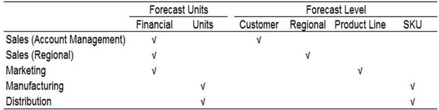
Figure 3-13. Examples of demand perspectives

It is clear that each division thinks of demand differently—while the supply chain organizations think in terms of specify products and locations, other organizations tend to perceive demand in aggregate terms. These differing views are an impediment to aligning demand and supply in a company. For example, sales may specify only the financial forecast for a region; since the supply chain organization needs to manufacture a product in order to meet the financial forecast, the financial numbers are converted into a unit forecast for each product. If the sales team is unaware of the specific product forecasts, situations can arise when sales meets financial projections, but with a product mix that is very different from what is being produced in the factories. The result is a mismatch between demand and supply.

While there is a need for organizational alignment, the solution is not to make all organizations think in terms of the stock keeping unit (SKU). Not only would that require a fundamental change in behavior; it would also reduce the benefit provided by the additional insight and perspective from the rest of the organization. Instead, the better solution, illustrated in Figure 3-14, is to rapidly reconcile the different viewpoints by aggregating and disaggregating demand to support the different perspectives.

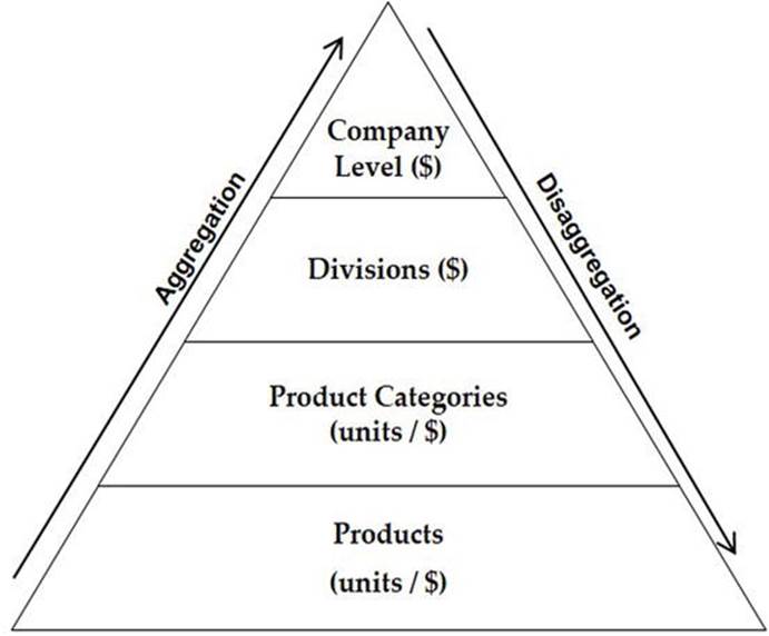
Figure 3-14. Pyramid forecasting

Categorization is a discipline that evaluates different ways of organizing demand in order to gain insight. Examples of different categories include:

· Product characteristics or attributes. This includes specific product features that can appeal to consumers. Examples are low-carbohydrate content in food items, portability for electronic goods, and sizes for apparel.

· Demographic characteristics. Geographic and economic segmentation, when combined with specific product characteristics, can provide unanticipated insight based on demographics. This can help with targeted marketing, promotions planning, as well as new product and new market forecasting. Examples include categorizing demand according to sales to different age groups.

· Production characteristics. Production modes can help identify trends related to customization and lead time preferences. A common example is build-to-stock versus configure-to-order for some electronic goods.

· Lifecycle characteristics. Yet another way to categorize products is based on demand patterns—for example, when a set of products is new or being phased out or when advertising is positively impacting demand. Such a categorization can be used to apply demand trends based on inputs from the marketing organization, and is an alternative method to the use of trend-based time series forecasts.

There are several benefits provided by a well-executed pyramid forecasting process, captured in Table 3-7. Implemented properly, the process will result in greater alignment between the different organizations, increase the sense of ownership of various aspects of demand, and improve visibility across products, product groups, and regions.

Table 3-7. Benefits Provided by Pyramid Forecasting

Feature	Description	Benefits
Interactive process	Demand inputs are collected from account representatives, sales managers, product marketing, channel fulfillment, and forecasters.	Involving several participants increases forecast accuracy and creates a company-wide sense of responsibility regarding demand goals.
Support for hierarchies	Revenue budgets, regional forecasts ($), and product-line forecasts ($, units) are all matched to SKU-level forecasts.	Allows participants to specify demand at levels that are natural to each. The different views are connected using hierarchies and aggregation/disaggregation rules.
Consensus- oriented	Mismatches between statistical forecasts and other numbers are highlighted and reconciled by involving the necessary individuals.	Reconciliation promotes alignments with the company, with “one forecast” driving its activities.

In conclusion, pyramid forecasting can benefit a company by promoting alignment among the different individuals and groups. Once the decision to initiate this process is taken, the following steps provide a guideline for implementation.

1. Identify demand perspectives and characteristics. Perspectives need to accommodate the requirements of the different organizations in the company, while characteristics provide a logical way to organize products in order to gain insights.

2. Specify rules for aggregation and disaggregation. While aggregation is a well-understood procedure, disaggregation requires some deliberation. For example, how should an increase in the revenue target for a product category be divided across the individual products? Commonly used methods include maintaining product-level ratios, favoring heavily promoted products, or favoring high-margin products.

3. Specify the steps to finalize the forecast. A mismatch between the numbers at any level in the hierarchy requires a review and reconciliation procedure that is acceptable to all parties.

4. Utilize software tools for efficiency. Develop or purchase software tools (such as spreadsheets or software applications) for gathering data, generating reports, and performing the reconciliation on a regular basis. While the use of simple spreadsheets may suffice for a few products, most businesses require systems to manage the process for many hundreds of products.

5. Ensure participation. The success of this forecasting process is dependent on the continued involvement of key managers from different organizations on a monthly basis.

6. Monitor performance. As the business environment changes and new products and customers are introduced, it may become necessary to modify perspectives, categories, and review procedures. Therefore, a periodic assessment (usually quarterly or semiannually) is important for the continued success of the process.

Forecasting Systems

When a company has several hundreds or thousands of products, the only viable approach is to perform the analysis frequently using a forecasting system. Some of the desirable factors of a forecasting system include the following:

· Support for defining different hierarchies for viewing demand, units, product categories, and the ability to aggregate and disaggregate demand according to specific rules.

· Ability to generate statistical forecast by applying time series methods. A good system will provide inbuilt ability to forecast at the SKU level, as well as at any of the group and characteristic levels defined above.

· Ability to include external data, such as economic indicators, for regression analysis at the SKU, group, or characteristic levels.

· Ability to combine two or more characteristics, and view demand and forecast for the combination. Such a feature can provide the analyst with valuable trend information related to specific product aspects that are of importance to customers.

· The ability to perform “what if” simulations, with users evaluating the impact of changes before broadcasting changes to the entire company.

Clearly, the complete set of system requirements will exceed the brief list shown above, and will need to consider specific product and industry considerations. It is recommended that each company follow a rigorous process of specifying the demand planning process and create an appropriate list of system requirements.

Demand Collaboration

The need for the communication of information between the retailer and the manufacturer has been mentioned in the previous discussions on distortion of demand. Collaborative planning, forecasting, and replenishment (CPFR)—the framework for this collaborative process and exchange of information mentioned in Chapter 1—has been proposed by the industry organization, Voluntary Interindustry Commerce Solution (VICS). The initial version of this process, then called collaborative forecasting and replenishment (CFAR), was initiated between Walmart and Warner-Lambert in 1995. The process allowed for sales and order forecasts for Listerine mouthwash products to be shared, with inconsistencies between the two numbers being highlighted. These inconsistencies were due to events such as Walmart promotions that had the capability of increasing demand significantly. Prior to the implementation of this process, Warner-Lambert, not being able to anticipate these swings, would maintain substantial inventory. The collaboration resulted in Walmart specifying orders six weeks in advance to match the six-week manufacturing lead time for Listerine. This allowed Warner-Lambert to smooth production and for Walmart to improve in-stock from 85 to 98% and reduce inventories by 25%.⁷

The CPFR model is divided into three phases—the planning phase, forecasting phase, and the replenishment phase. In total, there are nine steps in the process, summarized below.

The first two steps, termed the planning phase, are related to the development of the collaborative arrangement and the creation of the joint business plan. The agreement sets the objectives for the business partners and then defines the actions and necessary resources. It also identifies how the performance of the respective parties will be measured. The business plan specifies contract information for the products, including details regarding the minimum order quantity, order lead time, and the frequency of ordering.

The third through eighth steps are termed the forecasting phase. The third step in the process is to generate the sales forecast, based on the POS data and promotion planning. The fourth step is to identify exceptions to the sales forecast, based on the previously defined acceptance criteria. The fifth step is to collaborate and resolve these exceptions, and results in the generation of a new forecast. The sixth step is to create the order forecast, based on the sales forecast and inventory policies and destination for the products. The seventh step identifies exceptions to the order forecast, while the eighth step resolves these exceptions. The final step in the process is the replenishment phase, and results in the conversion of the order forecast into a firm order.

The CPFR model promotes structured communication between partners, a clear specification of the type and detail of information that needs to be communicated, and a platform for resolving differences. However, the implementation of CPFR can prove challenging in situations involving several thousands of products and locations, due to data issues and the manual effort required to manage numerous forecasts and exceptions. In response, companies have resorted to the use of fewer steps in order to simplify the process. Irrespective of the specific steps implemented, the value provided by collaboration in reducing inventories and increasing sales is indisputable.

Summary

Demand planning is the important process of specifying an accurate estimate of the market’s demand for a company’s products, and for ensuring that scarce supplies are utilized to meet demand in the best possible manner. This chapter has presented several methods for generating a demand forecast, including time series, collaborative, causal, and pyramid methods. The comparative advantages and disadvantages of these four methods are summarized in Table 3-8.

Table 3-8. A Comparison of Selected Forecasting Methods

Method	Advantages	Disadvantages
Time series	Easy to implement and update. “Grounded” in actual demand.	Forecast based on history, which is highly inaccurate when future demand is expected to deviate from past trends. Not effective in dealing with outliers.
Collaborative	Provides visibility into partners’ activities and enables alignment between companies.	Partners’ inputs can be biased and inaccurate and can distort demand information. Not easy to incorporate collaborative inputs with time series forecast.
Causal	Incorporate external information and leading indicators into forecast.	Requires insight into causal factors, which may be hard to establish. Data hungry. Effort required to set up and maintain model.
Pyramid	Provides mechanism for incorporating inputs from all sources in the company. Enables organizational alignment.	Forecasts from different sources can be qualitative and biased. Effort required to reconcile widely different views on demand.

Demand planning is not new—it has been performed in some manner by all businesses with or without the use of computers and sophisticated mathematics. However, this process will continue to evolve as new information becomes available, new ways of interacting with the customer are initiated, and novel methods to influence markets and the consumer are developed. A few developments that can have an impact on the demand planning process are:

· The increasing availability of new information related to economic trends and business activity. The growth in the use of the Internet allows for this information to be collected in an expeditious manner, which can increase the applicability and value of the information.

· The increasing use of radio frequency identification (RFID) to track movement of goods and sales. This technology provides a wealth of consumer-related information and can improve short-term forecast accuracy. However, challenges related to large data volumes and accuracy will have to be resolved before this becomes routine.

· Consumer loyalty programs that provide important information regarding preferences, buying patterns, and pent-up demand. The information collected can be used for forecasting, targeted marketing and promotions, and for influencing demand.

· Technological advancements that will result in new demand-fulfillment mechanisms. Such new methods have the promise of allowing businesses to reach consumers in a more direct manner and gain valuable insight into usage patterns.

Even as the availability of demand information grows and systems become more sophisticated, there is no perfect way to predict the future and forecast error cannot be eliminated. In fact, a forecasting process that remains unchanged over time will deteriorate in quality due to changes in the marketplace that invalidate one or more assumptions made by the models. Therefore, it is important that an adjustment procedure be used to align supply to changes in demand and make changes to model parameters (see discussions of such a procedure in Chapters 5 and 7). Attention to these different aspects of demand planning can help a company gain a better understanding of demand and the customer and thereby increase market share and profitability.

________________

¹S. J. Hoch, A. L. Montgomery, and P. E. Rossi, “Determinants of Store-Level Price Elasticity,” Journal of Marketing Research, Vol 32, Feb 1995.

²Frank Bass, “A New Product Growth Model for Consumer Durables,” Management Science, 15: 215-227, 1969.

³Demographic data from the U.S. Census Bureau, Census 2000.

⁴Martha Starr-McCluer, “The Effects of Weather on Retail Sales,” Federal Reserve Board of Governors, 2000.

⁵Revenue data from Lennox annual reports. Permit data from U.S. Census Bureau.

⁶H. L. Lee, V. Padmanabhan, and S. Whang, “The Bullwhip Effect in Supply Chains,” MIT Sloan Management Review 38 (3): 93-102, 1997.

⁷For additional information, see the VICS website and books on the subject such as Dick Siefert, Collaborative Planning, Forecasting and Replenishment: How to Create Supply Chain Advantage (McGraw Hill, 2006).