The Profitable Supply Chain: A Practitioner’s Guide (2015)

Chapter 7. Supply Chain Performance Review

Performance review is an important activity in the plan-do-check-act (PCDA) management philosophy for maintaining operating efficiency and enabling continuous improvement. The review process is especially involved for SCM, given the breadth of activities across manufacturing, procurement, transportation, and distribution. This chapter provides the reader with an overview of operational and financial metrics for these different segments and a process framework for implementing the review process.

The Importance of Reviewing Performance

The change in the structure of the company to include global suppliers and customers has required an associated modification to the way in which ­performance is reviewed and acted upon. What used to be a casual meeting of managers to discuss operations at a collocated manufacturing plant has grown to virtual meetings between executives at several companies in different continents. Additional changes, including product proliferation, have added to the complexity of gathering data and assessing performance. The following extracts from an annual report of Hauppauge, a consumer electronics manufacturer, emphasize some of the challenges:

Volatility of gross profit percentage: Over the eight quarters ended with the fourth quarter of fiscal 2007, the gross profit percentage has ranged from a low of 18.79% to a high of 22.79%.

The company emphasizes the gross profit range of 4% and proceeds to highlight the demand-side variables that cause this volatility:

Factors affecting the volatility of our gross profit percentages are:

· Mix of product. Gross profit percentages vary within our retail family of products as well as for products sold to manufacturers. Varying sales mix of these different product lines affect the quarterly gross profit percentage

· Fluctuating quarterly sales caused by seasonal trends. Included in cost of sales are certain fixed costs, mainly for production labor, warehouse labor and the overhead cost of our Ireland distribution facility. Due to this, when unit and dollar sales decline due to seasonal sales trends these fixed costs get spread over lower unit and dollar sales, which increase the product unit costs and increase the fixed costs as a percentage of sales.

· Competitive pressures. Our market is constantly changing with new competitors joining our established competitors. These competitive pressures from time to time result in a lowering of our average sales prices which can reduce gross profit.

Next, the company lists a few of the supply-side variables contributing to this volatility:

· Supply of component parts. In times when component parts are in short supply we have to manage price [raw material cost] increases. Conversely, when component parts’ supply is high we may be able to secure price decreases.

· Sales volume. As unit sales volume increases we have more leverage in negotiating volume price [raw material cost] decreases with our component suppliers and our contract manufacturers.

· Cost reductions. We evaluate the pricing we receive from our suppliers and our contract manufacturers and we often seek to achieve component part and contract manufacturer cost reductions.

· Volatility of fuel prices. Increases in fuel costs are reflected in the amounts we pay for the delivery of product from our suppliers and the amounts we pay for deliveries to our customers. Therefore increasing fuel prices increase our freight costs and negatively impact our gross profit.

Managing product mix through market strategy and new products, moderating seasonal trends, efficiently managing shipments and achieving cost reductions are a company priority and are critical to our competitive position in the market. Although our goal is to optimize gross profit and minimize gross profit fluctuations, in light of the dynamics of our market we anticipate the continuance of gross profit percentage fluctuations.

—2007 Annual Report, Hauppauge, Inc.

While several of the factors listed above are fluctuations due to the economic or competitive climate, the company also talks about its continuous improvement initiatives related to raw material costs and contract manufacturer cost reductions. This two-pronged approach—first to sense and react to unforeseen factors and minimize profit fluctuations, and second to constantly evaluate options to lower costs—is required for improving performance effectively.

The list of areas that require attention is different by industry, by company, and even by product line. This need to tailor measurements by product lines is driven by the level of maturity—whether the product is being introduced, has reached maturity, or is in the process of being phased out. This requires that the company focus on a different set of drivers as time progresses, as shown in Figure 7-1. The figure illustrates that supply chain drivers such as flexibility and costs increase in importance as the company matures, and the ability to deliver products in a timely and profitable manner are of primary concern.

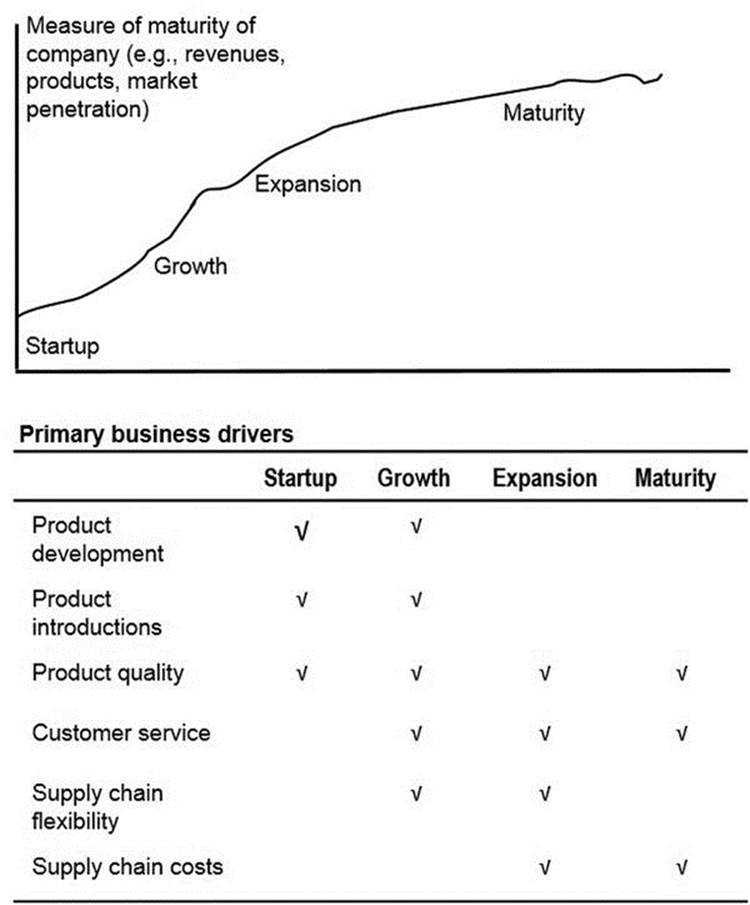
Figure 7-1. Focus areas for various stages of product maturity

The performance of the supply chain can be assessed by its impact on customer service, flexibility, and costs. Customer service refers to the ability to meet the expectations of the customer in order to be a leader or remain competitive in the marketplace. Specific measures include the quoted response time for satisfying customer demand and the ability to meet these commitments.

Flexibility is important when the company is in its growth phase and is introducing new products or entering new markets. The associated uncertainty in estimating demand can result in orders that are very different from the original assumptions. If the company is to sustain its growth phase and increase market penetration, it needs to satisfy these unanticipated orders in a timely manner, which requires flexibility in the supply chain. Common measures of flexibility include lead times for raw material and production and utilization of manufacturing capacity.

Supply chain costs increase in importance as the company's sales increase and the need to operate a profitable business becomes the primary goal. Due to the multitude of activities that contribute to costs, there are several metrics that need to be tracked, including manufacturing costs, overhead, and inventory obsolescence.

Challenges faced when attempting to measure or improve the performance the supply chain include the following:

· Difficulty in handling the large volume of data generated by several hundreds or thousands of items across factories, distribution centers, and suppliers. Any relationships between items, as with parts used to manufacture products, further increases the complexity of data.

· Difficulty in identifying and analyzing issues due to the expansiveness of the supply chain. With the gradual departure from vertical integration, operational issues can occur in the sales channels (retailers or distributors) or at contract manufacturers, key suppliers, and transportation providers.

· Difficulty in aligning differing viewpoints that arise due to the involvement of multiple parties in the review process. A lack of agreement or clarity as to how performance needs to be measured can make the process ineffective. In fact, when metrics are acted upon in isolation, it is possible for results to be detrimental to the overall performance of the business. This can be seen from the example of reducing use of expensive overtime labor, only to find that service levels have been excessively impacted. Therefore, it is necessary to examine metrics in a holistic manner in order to get a complete understanding of a situation.

The rest of this chapter examines several of these challenges. A review of existing frameworks for performance assessment is provided, followed by a description of a process for performance management and a section on metrics lists measurements for tracking and reducing margin volatility. The final section provides a framework for continuous improvement.

An Overview of the SCOR Model and Metrics

Metrics, also referred to key performance indicators (KPIs), are important indicators of performance. Metrics can be organized according to the business drivers discussed at the beginning of the chapter (customer service, flexibility, and costs) or by function (inventory, manufacturing, transportation, procurement, and supply chain). The advantage of organizing metrics according to functions is that the alignment with company roles clarifies responsibilities.

A widely-used framework for defining metrics is the Supply Chain Operations Reference (SCOR) model, developed by the Supply Chain Council.¹ This model divides metrics into many levels, based on the amount of detail (with level 1 representing the highest level and level 3 representing the detailed measurements). At the highest level, metrics are organized according to three categories: customer-facing, internal-facing, and shareholder-facing.

· Customer-facing metrics include delivery performance, fill rates, and perfect order fulfillment. Each of these is further decomposed into more detailed metrics. For example, the detailed metrics for delivery performance are supplier on-time and full delivery, manufacturing schedule attainment, warehouse on-time and in-full shipment, and transportation provider on-time delivery. Other customer-facing metrics are order fulfillment lead time, supply chain response time, and production flexibility. The last two metrics measure the ability of the supply chain to respond to unplanned events. The response time measures the number of days taken to respond to an increase or decrease in demand without incurring additional costs. Production flexibility measures the number of days to achieve a 20% increase or decrease in orders without incurring cost penalties.

· Internal-facing metrics are divided into two categories—costs and asset management efficiency. Cost metrics include cost of goods, total supply chain management costs, value-added productivity, and warranty/returns processing costs. Value-added productivity refers to direct margin (obtained by subtracting revenue from direct costs and dividing by the number of employees). Supply chain asset management efficiency metrics include cash-to-cash cycle time, inventory days of supply, and asset turns.

· Shareholder-facing metrics are divided into three categories—profitability, effectiveness of return, and share. Profitability metrics include gross margin, operating income, net operating income, and economic profit. Effectiveness-of-return metrics include return on assets, return on sales, and return on investment. Share metrics include ­earnings per share (EPS), EPS percentage change in a ­twelve-month period, and stock price percentage change in a ­twelve-month period. Shareholder-facing metrics are well-understood and -reported financial measurements and ratios.

The SCOR framework was created collaboratively by a working group of research institutions, companies from several industries (including electronics, semiconductor, aerospace, and consumer goods), and consulting and software entities. Therefore, one of the advantages is that significant thought and effort has been invested into the specification, and this framework has been implemented by many of the participating companies. However, this method of preparation has also created a challenge: the specification is very broad since it needs to accommodate a wide variety of companies. The result is that considerable effort is required to select a suitable set of metrics and specify data requirements and calculations. This problem is not specific to the SCOR model, but is inherent in all frameworks that attempt to standardize data, measurements and metrics.

The metrics and methods presented in this chapter leverage these frameworks for analyzing performance of manufacturing, procurement, distribution, and supply chain operations. But selecting appropriate metrics and supporting measures is only the first step in designing the review process; equally important is the presentation of the information in a way that is easy to assimilate, and the specification of a rigorous approach towards understanding causes and initiating actions. Therefore, this chapter provides details regarding metrics, reports and procedures for conducting the performance review.

The Performance Review Process

The review process is geared towards monitoring all aspects of the supply chain, shown in Figure 7-2. The first step in the process is to collect the necessary data related to manufacturing, procurement, distribution, and transportation. The second step is to analyze variances between actual performance and targets in order to reduce margin volatility. The third step is to analyze the relative performance of products, sites, and suppliers in order to identify candidates and areas for continuous improvement. Finally, any actions involving changes to targets, replenishment policies, forecasting methods, and inventory policies are implemented.

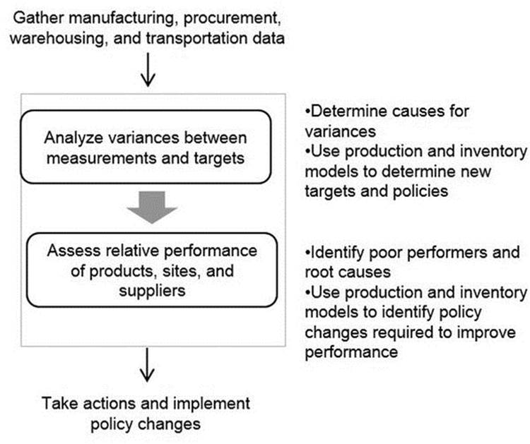
Figure 7-2. The Performance Review process

Metrics, Variance Analysis, and Diagnostic Procedures

Each of the functional areas—manufacturing, procurement, distribution, transportation, and supply chain—are analyzed according two aspects: operational performance and financial performance. Measurements are organized along the same lines, with operational metrics gauging the ability of a particular function to support the delivery of products, and financial metrics gauging the ability to perform the function in a cost-effective manner.

Once operational and financial metrics have been defined, the next step is to compare performance relative to a baseline, either a target or performance in a prior period, or both. This comparison is referred to variance analysis, and is an important step in understanding the causes for a deterioration or improvement in performance. An example of this procedure is seen from the following except from an annual report of Cisco:

Product gross margin for fiscal 2010 increased by 0.2 percentage points compared with fiscal 2009, due primarily to lower overall manufacturing costs driven by strong operational efficiency in manufacturing operations, value engineering and a reduction in other manufacturing-related costs. Value engineering is the process by which production costs are reduced through component redesign, board configuration, test processes, and transformation processes. The product gross margin for fiscal 2010 also benefited from the increase in shipment volume. A favorable product mix contributed slightly to the increase in product gross margin percentage. Fiscal 2010 product gross margin was negatively impacted by sales discounts, rebates and product pricing, which were driven by normal market factors, as well as the geographic mix of product revenue. The impact from sales discounts, rebates and product pricing was within our expected range.

—2010 Annual Report, Cisco Systems, Inc.

The annual report also provides a graphic to represent the variance discussion above. The graphical and textual variance analysis provided by Cisco helps describe the business environment and the company’s measure of efficiency in reacting to changes. In this chapter, a similar approach towards variance analysis is provided at a detailed level for each of the functions.

Metrics are further categorized as primary or diagnostic. Primary metrics are the most important measures of performance, while diagnostic metrics are supporting measurements that help diagnose the causes for variances in the primary metric. Delivery lead time is an example of a primary metric, while capacity utilization is a diagnostic metric that can be used to clarify whether a deterioration in the delivery lead time is due to insufficient capacity.

Manufacturing

The primary operational metric is manufacturing delivery performance. It measures the timely completion of orders and is an assessment of internal efficiency as well as a customer service metric for make-to-order companies. Delivery performance is calculated according to Equation 7-1:

Reasons for deterioration of delivery performance include insufficient capacity, high reject rates (poor quality), or an increase in downtime. These different aspects can be combined into a single measurement called overall equipment effectiveness (OEE). OEE has three components: availability, performance, and quality. Availability is the percentage of scheduled time that a resource is available to operate and takes into account any time lost due to downtime (Equation 7-2). Downtime measures hours lost and might be due to any of several reasons, including machine repair or lack of availability of material for processing.

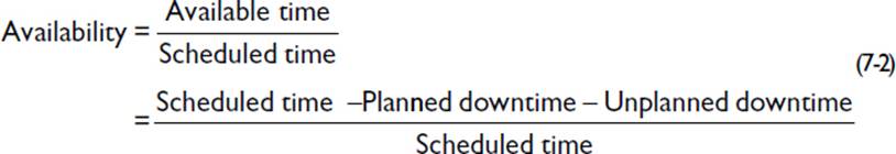
For example, if a work center is scheduled to run 8-hour shifts for 25 days in a particular month, then the scheduled time is (8 * 25) = 200 hours. If the 8-hour shift includes a 30-minute lunch break, then the planned downtime is (0.5 * 25) = 12.5 hours. In addition, if the unplanned downtime during the month is 27.5 hours, the total downtime is (12.5 + 27.5) = 40 hours. As a result, available time is (200 – 40) = 160 hours, and the Availability is (160 / 200) = 80%.

The next component of OEE is performance, which captures the speed at which the work center is operating, according to Equation 7-3:

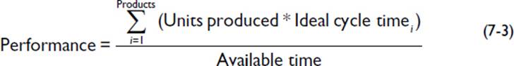
For example, consider a month in which three products are in a work center. The units produced are 125, 250 and 350 units, and the targeted cycle times are 20, 15, and 10 minutes, respectively. With available time of 160 hours, the performance metric is calculated as

Therefore, performance is calculated to be 101.5%, indicating that the cycle time for the work center was better than targeted.

The final component of OEE is quality, which captures the effect of defects and rejected parts, according to Equation 7-4:

Continuing the example, if the units started for the month for all three products are 750 and the resulting good units produced are 725 units, the quality metric = (725 / 750) = 97%.

Once these three components of the OEE have been calculated, the overall metric is:

For the work center, OEE is (0.8 * 1.015 * 0.97) = 0.79 (i.e., 79%). When these values are compared with prior performance, inferences can be drawn regarding areas that cause the deterioration in performance. An example of this variance analysis is shown in Table 7-1. The variance analysis helps identify availability of the mounting work center as the cause of deterioration in delivery performance. Since availability is affected by unplanned downtime, a further analysis of machine maintenance or availability of raw materials would help narrow down the causes and the appropriate remedial actions can be taken (such as replacing work parts or increasing safety stocks for raw materials).

Table 7-1. Operational Metrics for Manufacturing

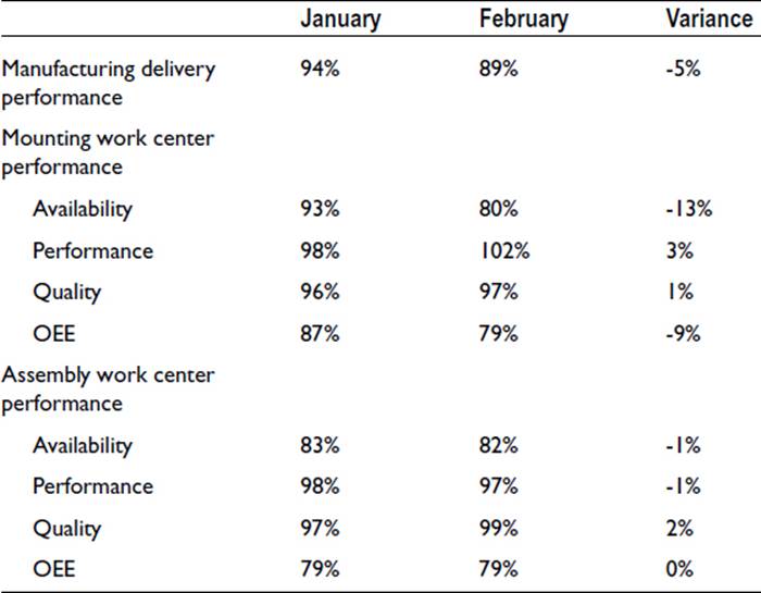
The financial metric for manufacturing is cost as percentage of revenue, and diagnostic metrics are costs related to labor costs, maintenance, direct materials, and overheads. For each of these sections, it is useful to track costs as a percentage of revenue as well as per unit, as shown in Table 7-2. In the example, the current month’s performance (February) is compared to the prior month, and the variance is calculated as the February value minus the January value. The manufacturing spend as a percentage of revenue has increased by 4%, and unit costs have increased by $2.89. The rest of the table helps analyze this variance. The increase is due to labor, direct materials, and overhead. Along with hours, the labor section also lists the two other OEE components—availability and performance—as supporting measurements, which reveal that the variance is largely due to availability.

Table 7-2. Financial Metrics for Manufacturing

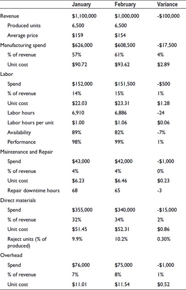
Availability can be further analyzed by reviewing the downtime measurement in the maintenance and repair section of Table 7-1, which reveals that the lack of availability does not appear to be due to unavailability of machines. Therefore, the analyst needs to evaluate other causes affecting availability, such as lack of raw materials and inventory buffers or poor scheduling of resources. Also, overheads contribute to the variance due to fixed costs being distributed across fewer units, such that there is only a 1% increase as percentage of revenue yet almost a 5% increase in unit overhead cost.

Procurement

The primary operational metric is supplier delivery performance, which is a proxy measurement of the time taken to receive material from the supplier once the order has been placed. The calculation in Equation 7-6 is based on the number of shipments that have been delayed:

Alternatively, on-time performance may be tracked, based on the number of units delayed or the cost of materials delayed.

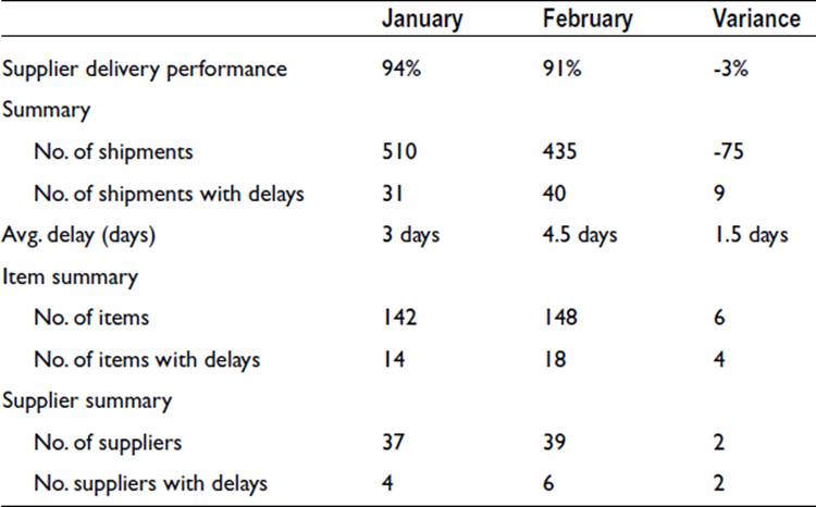
Reasons for delays include introduction of new suppliers or parts, significant increase in purchasing volume from a supplier, or issues at a supplier's plant. The corresponding diagnostic metrics can be tracked in a single view to highlight issues and reasons, as shown in Table 7-3. The summary section lists the number of delayed shipments and the average delay, and the monthly comparison shows that performance has deteriorated. The item summary section lists the number of items procured in each month, with the increase indicating that new items were ordered. Similarly, the supplier summary section indicates that two new suppliers were added. On the basis of this report, further analysis is warranted, with specific attention to the newly added items and suppliers.

Table 7-3. Operational Metrics for Procurement

The financial metric for procurement is material cost as percentage of revenue. In addition, each item can be analyzed according to the purchase price variance, which is the difference between the actual and standard unit price for an item (Equation 7-7):

The purchase price variance may be calculated for each item and supplier and is a useful metric to highlight price increases. If the increases are due to expediting costs, corrective actions such as increasing safety stocks or communicating changes quickly can help to reduce the variance. If the increases are due to price hikes by the supplier, contractual terms or alternate sources of supply can be evaluated.

Transportation

The primary operational metric is transportation delivery performance, measured as the number of late deliveries in comparison to total deliveries (Equation 7-8):

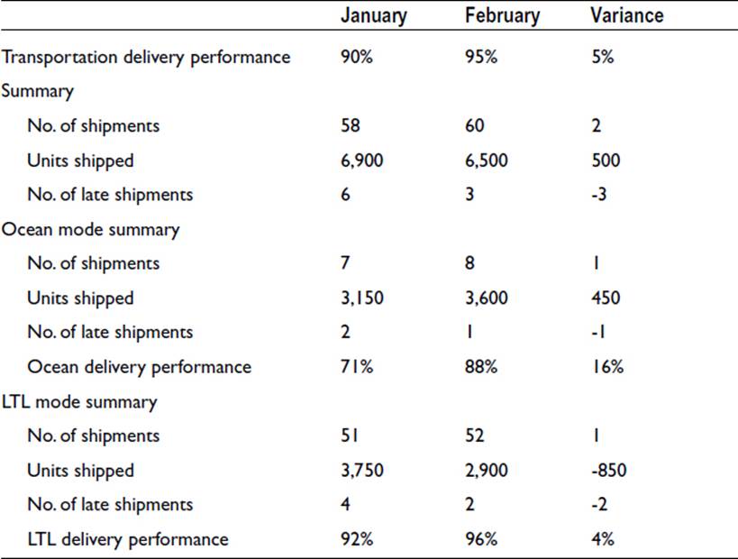
If multiple modes of transportation are used to transport goods from manufacturing plants to distribution centers, then delivery performance needs to be analyzed by mode, as shown in Table 7-4 for two modes of transportation: ocean and trucks (where LTL mode stands for “less-than-truckload” shipping). The performance improvement shown in Table 7-4 is seen to be attributable largely to a lower delay in ocean shipments.

Table 7-4. Operational Metrics for Transportation

Factors contributing to deterioration in delivery performance include the following:

· Loading delays due to miscommunication between supplier or manufacturer and the transportation provider

· Increased handling complexity for new products or material, resulting in additional time to turnaround trucks

· Missing paperwork, including documents required for clearing customs

· Delays in consolidation truckloads

· Lack of timely availability of transportation resources

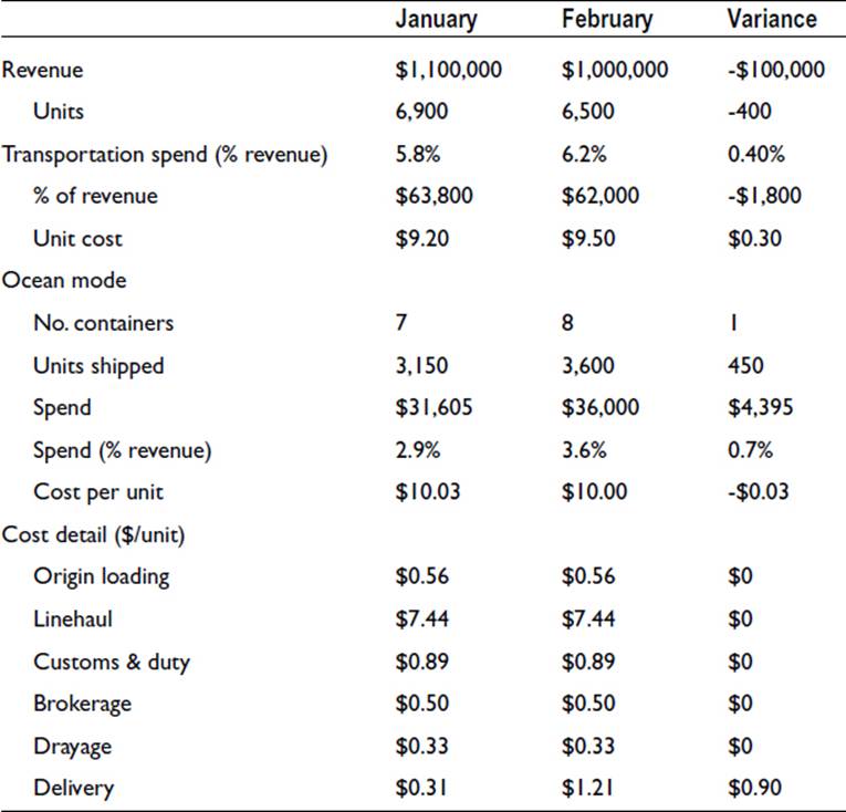
The financial metric for transportation is transportation cost as percentage of revenue. As with delivery performance, financial performance also needs to be analyzed by mode so that specific transportation providers and processes can be addressed. An example of this performance review is shown in Table 7-5 for a single mode of transportation (ocean containers). In the example, transportation spend as a percentage of revenue has increased from February to March by $0.30 per unit. The mode analysis indicates that the increases are due to ocean shipment charges, driven by an increase in delivery charges. The next step is to examine the delivery leg in detail to understand the reason for cost increases. This template can be extended to additional modes of transportation, such as truckload or rail, as well as additional cost lines that will need to be added for different modes and provider contracts.

Table 7-5. Financial Metrics for Transportation

Supply Chain

Operational metrics for supply chain are (a) fill rates and out-of-stock for build-to-forecast companies and (b) order fulfillment time for build-to-order companies.

Fill rates measure the ability of a company to fill customer orders in a timely manner, usually from onhand inventory. There are many versions of the fill rate metric which are applicable to different supply chain configurations, a few of which are described below.

Value fill rate is the financial value of order lines shipped on time, calculated as follows:

Note that this metric applies a lower penalty for delayed shipments of low-value products.

Another version is the SKU fill rate, which performs the calculation based on the number of products shipped on time, as follows:

The SKU fill rate penalizes all units equally, irrespective of the value of the units delayed.

Yet another variation is the line count fill rate, which simply measures the number of lines in the first shipment relative to the total number of lines in the order.

For a company that ships its product in cases, a popular variation is the case fill rate, which measures the number of cases in the first shipment relative to the total number of cases ordered.

The selection of a specific fill rate calculation depends on the nature of the business and relationship with the sales channels. If the customer (retailer) assesses delivery performance based on the number of units delivered in a timely manner, the SKU fill rate is to be used. However, if the customer is a distributor and does not penalize for late deliveries, the manufacturer may choose to use the value fill rate to estimate lost revenue.

The assessment of product availability in a retail environment is based on out-of-stock (OOS) events. An OOS situation is one in which a consumer is unable to find a specific product on a retail shelf. Because an OOS represents a lost sale, it is an important metric for the retailer. It is also becoming increasingly important for manufacturers because the lost opportunity is greater. Although retailers may not lose revenue if a substitute product from another manufacturer is available for the customer, manufacturers lose the entire proceeds due to unavailability.

Both OOS and fill rates measure product availability and the customer experience. Fill rates are appropriate when responding to customers' purchase orders; whereas OOSs are appropriate when demand needs to be satisfied immediately, as shown in Figure 7-3.

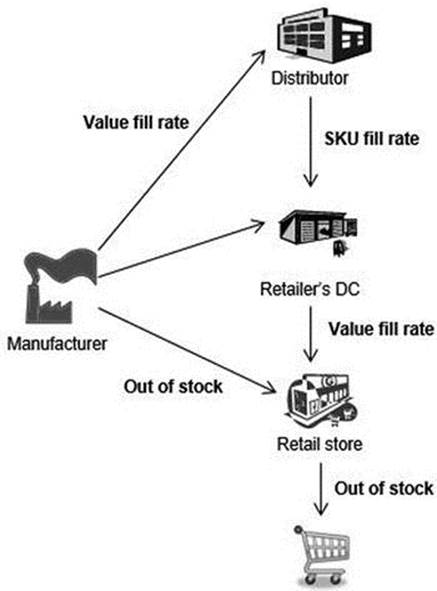
Figure 7-3. Fill rates and out-of-stock metrics for various business environments

OOS measurements are not easy to perform if inventory reviews are done on a periodic basis, because it is difficult to determine the duration for which the product was unavailable. Recent advances in the use of perpetual inventory systems that utilize scan data to keep track of sales allow for better measurements. Once the time at which an item goes OOS is determined, it can be used to calculate the duration for which the OOS occurs (i.e., until the next replenishment occurs). The OOS metric is then calculated as the OOS duration divided by the time between replenishments. Common reasons for OOS include the following:

· The product is in the back room but not in the shelf.

· The shelf space allocated to the product does not match its rate of consumption (demand) and replenishment schedule.

· Insufficient inventory exists in the supply chain (that is, at the retailer’s distribution center or with the manufacturer).

Diagnostic measures that can support OOS analysis include shelf space allocation to address the issue of inadequate shelf space and a review of the inventory policy. Shelf place allocation can be calculated according to Equation 7-11:

For example, if the number of units of an item replenished every 3 days is 30 and the expected demand over these 3 days is also 30 units (at 10 units per day), then the shelf space allocation is calculated to be 1, indicating that sufficient space exists for the expected demand.

Equation 7-11 results in only 50% service levels. If 95% service levels are desired, the service-level method described in Chapter 2 can be used to modify the calculation, as shown below in Equation 7-12:

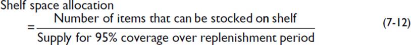
In Equation 7-12, supply for 95% coverage is calculated as the expected demand over the {replenishment period + [1.65 * (standard deviation of forecast error)]}.

In the previous example, if the standard deviation of demand is 2 units per day, the standard deviation over the replenishment is (Square root(3) * 2) = 3.5 units, and the denominator is [30 + (1.65*3.5)] = 36 units. This results in a shelf space allocation of (30/36) = 83%, indicating that shelf space is insufficient.

The inventory policy in use can be studied in a similar manner. If a periodic review is performed, then the order-to-level is set equal to the supply for 95% coverage over the replenishment period, and the order quantity is determined accordingly.

A broader view of diagnosing fill rate issues requires analyzing demand variability and supply or safety stock issues. Forecast accuracy is the most important single metric for gauging the effectiveness of the forecasting process. The most common metrics for measuring forecast accuracy—mean absolute percentage error (MAPE), mean absolute deviation (MAD), root mean square error (RMSE), and forecast bias—were described in detail in Chapter 3.

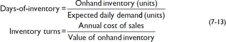
Inventory or safety stock metrics include days-of-inventory and inventory turns, defined as follow:

The first step in the diagnostic procedure is to review inventory levels. If these levels are low, then an analysis at a product or item level is required to determine whether low supplies are due to manufacturing or supplier issues.

If sales are higher than the demand forecast, a lack of forecast accuracy contributes to the deterioration in fill rates. The first step in analyzing forecast error is to examine the bias. Determination of a biased qualitative forecast requires the forecaster to take corrective steps such as attaching a lower level of confidence to sales inputs or multiplying the forecast by a corrective factor. Such a determination further requires the forecaster to examine the data to identify changes in the underlying trends and seasonal factors and to adjust the forecasting parameters accordingly.

After reviewing for bias, the next step is to check for forecast distortion. If it is found, the responsible customers and account representatives must be contacted, the causes identified (such as one-time demand or replenishment policies), and the appropriate adjustments made. Finally, if the number of outliers is increasing, then causal factors need to be identified and incorporated into the forecasting process.

It is possible for both demand and supply measurements to be adequate, indicating that the inventory policy and model being used are not performing satisfactorily. Underperformance might be caused by departures from some of the underlying assumptions, such as the nature of the demand distribution and demand correlation. In such cases, the model may need to be modified or the target service level increased to compensate for these unknown factors.

One of the difficulties in performing the above review and analysis is that fill rates may not be captured accurately, as often proves the case with high-value sales and strategic customer accounts. For example, if a salesman is aware of low inventory levels for a particular product and guides a customer toward the purchase of an alternate product, calculations based on sales and inventory will fail to capture this shortfall. In fact, the data can lead the analyst to believe that the inventory planning process is performing adequately, which can be contrary to the belief of the rest of the organization and the company's customers. In such situations, it is necessary to augment the quantitative measurement with surveys and interviews with the sales and marketing division and with channel partners. Any perception that a particular product is always in short supply needs to be considered while setting inventory parameters and safety stock levels.

Financial Metrics for Supply Chain

The financial metrics for the supply chain are cost of goods sold (COGS) and gross margin return on operating assets (GMROOA). Cost of goods include all direct costs, including production, raw materials, transportation, and storage. The equation for GMROOA is shown below.

Examples of a COGS analysis and GMROOA analysis are shown in Table 7-6. The “cost detail” section of the table summarizes the cost contribution from the different sections of the supply chain. In this example, unit costs have increased for raw materials, production, and transportation. The cost variance for each line may be further analyzed, based on the procedure described previously for manufacturing, procurement, and transportation functions.

Table 7-6. Financial Metrics for the Supply Chain

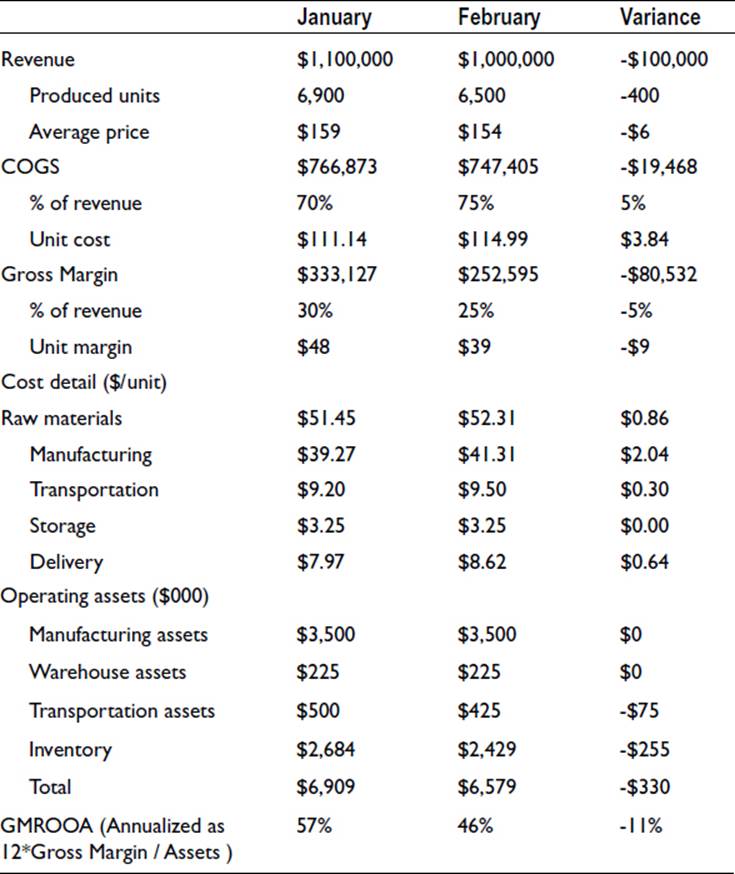
Operating assets include all assets used for generating revenues, including fixed assets such machinery in the plants and distribution centers, transportation assets owned by the company, and nonfixed assets such as inventory. For the purposes of measuring the efficiency of the supply chain, cash that is not required to operate the business is not included in the operating asset calculation. GMROOA is a measure of the efficiency with which a company utilizes its investment to make a profit, such that a higher value indicates better performance. It is a useful measure for comparing the performance across product lines, divisions, and companies. GMROOA can be increased by either increasing gross margin or by decreasing operating assets.

In addition to these operational and financial metrics, the supply chain organization needs to be evaluated on the basis of the speed and effectiveness of completing tasks related to demand and supply coordination activities. This is the time taken to complete the planning cycle, consisting of planning (demand, inventories, production, shipments, and purchases) and communicating with suppliers and customers. This measure of planning cycle time is a combination of the systems and manual steps required to complete the plan. It is especially important in dynamic environments in which demand and supply situations may change frequently.

The cost of operating the supply chain department also needs to be evaluated. The supply chain management overhead includes the following costs:

· Salaries for demand, inventory, production planners and executives

· Facility costs for supply chain personnel

· Travel costs for managing the different facilities

· Maintenance and support costs for supply chain systems

Industry rates for this overhead cost vary between 0.5% and 3% of revenue, depending on the nature of the business and the complexity of the operations. Of greater significance than the absolute value is the trend of these costs over time, which should be monitored to ensure a flat or downward trend in costs relative to revenue. If this metric spikes following an expensive systems implementation, it needs to be justified by a corresponding reduction in unit costs or increase in fill rates.

Continuous Improvement

Companies are constantly looking for ways to deliver additional margins and shareholder value. A continuous improvement program is one of the most important efforts in delivering on this objective. The preceding section described metrics for tracking performance for a product across time periods in order to identify and address any deterioration. This section compares the relative performance of products, suppliers, and customers in order to identify underperformers and rationalize the portfolio. Such a relative comparison becomes increasingly important as a company grows in size. Large companies may have over hundreds of thousands of products and thousands of suppliers and customers. On account of this proliferation, there are frequent opportunities to phase out underperforming products, reduce the reliance and spend on underperforming suppliers, and change pricing and fulfillment terms with low-margin customers.

Product Performance and Rationalization

The primary reason for evaluating the relative performance of products is product proliferation, which may result from the following factors:

· Global presence, requiring different sets of products to satisfy variations in local demand

· Products not being phased out after the introduction of “replacement” products

· Sales incentives geared towards revenue targets, which rewards salespeople's accommodation of customer choice in product configuration

· Mergers and acquisitions resulting in redundant or overlapping product lines

· Special accommodations for different customers’ packaging requirements or languages

Consider the following excerpt from an annual report of Levi Strauss, an apparel manufacturer:

Trends Affecting our Business: Brand and product proliferation continues around the world as we and other companies compete through differentiated brands and products targeted for specific consumers, price-points and retail segments. In addition, the ways of marketing these brands are changing to new mediums, challenging the effectiveness of more mass-market approaches such as television advertising.

Quality low-cost sourcing alternatives continue to emerge around the world, resulting in pricing pressure and minimal barriers to entry for new competitors. This proliferation of low-cost sourcing alternatives enables competitors to attract consumers with a constant flow of competitively-priced new products that reflect the newest styles, bringing additional pressure on us and other wholesalers and retailers to shorten lead-times and reduce costs. In response, we must continue to seek efficiencies throughout our global supply chain.

—Levi Strauss & Co., 2010 Annual Report

This proliferation trend is seen in almost all consumer-oriented industries, including apparel, footwear, electronics, and consumer durables. The need to constantly evaluate the product offering in order to weed out underperformers is emphasized in the following excerpt from an annual report Bausch & Lomb, a contact lens manufacturer:

We pioneered the development of soft contact lens technology and are one of the largest manufacturers of contact lenses in the world. Our product portfolio is one of the broadest in the industry and includes traditional, planned replacement disposable, daily disposable, multifocal, and toric soft contact lenses and rigid gas permeable (RGP) materials. These products are marketed by our own sales force and through distributors to licensed eye care professionals and health product retailers.

Net sales of contact lenses constituted 31 percent of our total revenues in fiscal year 2006, and declined 3 percent from the prior year. Overall strong double-digit growth in our PureVision lines of silicone hydrogel contact lenses was more than offset by lower sales of two-week spherical contact lenses in Japan (reflecting overall market trends), SofLens Toric disposable contact lenses (resulting from the continued roll-out of PureVision Toric in the U.S. market), collateral negative impact on our Asian contact lens business resulting from the MoistureLoc recall, and lower sales of older technology products (reflecting ongoing product rationalization initiatives).

—Bausch & Lomb Inc., 2009 Annual Report

The traditional method for identifying underperformers is to create a Pareto chart of revenue contribution, with the bottom fraction being candidates for rationalization. Following this analysis, the analyst interviews the engineering and marketing organizations and customers regarding the value provided by these products, and any products that are so identified as unnecessary become candidates for phase-out.

This simple method for identifying underperformers can however be misleading. For example, a product might have been recently introduced and its sales might still be ramping up. Or a product might contribute insignificantly towards revenues yet still be highly profitable. It is therefore necessary to identify better gauges of product performance. One such metric is the gross margin return on inventory (GMROI). Two forms of this return-on-assets measure, which considers only the inventory investment, are defined as follows:

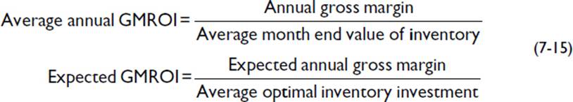
The average annual GMROI is the actual measurement, based on annual sales and on-hand inventories. (The analyst may alternatively calculate monthly or weekly returns.) Expected GMROI is based on expected values of gross margin, calculated from the inventory models described inChapter 2.

Challenges in measuring average annual GMROI include the following:

· Capturing costs accurately. Gross profits for a product need to reflect the true cost associated with producing, transporting, storing, and delivering the product. However, many companies often do not capture costs with adequate detail to support this view. For example, overtime labor costs may be incurred in order to satisfy an unanticipated order for a single product, but if the company simply allocates labor costs for the entire week, then the additional cost will be spread across all products, which can distort the margin estimation.

· Tracking inventory accurately. On-hand inventory used in calculating GMROI is often based on an end-of-week or end-of-month recording. However, shipments may be received into inventory according to a different schedule. Consider, for example, a distribution center that receives shipments sporadically. In one week, a shipment is received to cover two weeks of demand, which will result in high inventory levels the first week but far lower levels the following week. The measured GMROI for these two weeks will be very different.

Averaging inventory values over several weeks will partially address the second issue but create the different problem that any upward or downward trends will be masked and not discovered for several weeks. Owing to these measurement challenges, the expected GMROI is a better measure for comparing product performance. In this equation, calculate expected annual gross margin by the methods described in Chapter 2 for the Newsvendor or Incremental Margin models. Then perform product rationalization by Pareto analysis on the GMROI values.

Supplier Performance and Rationalization

Product breadth combined with multinational presence has resulted in a proliferation in the number of suppliers from which a company sources its products. For example, the home improvement retailer Lowe's sources products from more than 7,000 vendors worldwide (2013), and retail giant Walmart has more than 60,000 vendors. Supplier proliferation may also occur in result of acquisitions and mergers, or when engineering teams within a company fail to collaborate on sourcing decisions. The following excerpt from an Estée Lauder annual report provides several important reasons for rationalizing the supply base:

The principal raw materials used in the manufacture of our products are essential oils, alcohol and specialty chemicals. We also purchase packaging components that are manufactured to our design specifications. Procurement of materials for all manufacturing facilities is generally made on a global basis through our Global Supplier Relations department. We are making a concentrated effort in supplier rationalization with the specific objective of reducing costs, increasing innovation and speed to market and improving quality. In addition, we continue to focus on supply sourcing within the region of manufacture to allow for improved supply chain efficiencies. As a result of sourcing initiatives, there is increased dependency on certain suppliers, but we believe that our portfolio of these suppliers has adequate resources and facilities to overcome any unforeseen interruption of supply. In the past, we have been able to obtain an adequate supply of essential raw materials and currently believe we have adequate sources of supply for virtually all components of our products.

We are continually benchmarking the performance of the supply chain and will change suppliers, and adjust our distribution networks and manufacturing footprint based upon the changing needs of the business. As we integrate acquired brands, we continually seek new ways to leverage our production and sourcing capabilities to improve our overall supply chain performance.

—Estée Lauder Companies Inc., 2010 Annual Report

The company emphasizes that several benefits accrue from supplier rationalization. Costs can be reduced because increasing the quantity purchased from a smaller supply base can be used to negotiate better prices. Also, increasing the reliance on suppliers who are more inclined to invest in research can help increase innovation. Therefore, it is important for a company with a diverse supply base to clearly communicate metrics and targets to its suppliers so that performance can be evaluated on a periodic basis.

This view is likewise emphasized in an annual report of the Intel Corporation, a semiconductor manufacturer:

We have thousands of suppliers, including subcontractors, providing our various materials and service needs. We set expectations for supplier performance and reinforce those expectations with periodic assessments. We communicate those expectations to our suppliers regularly and work with them to implement improvements when necessary. We seek, where possible, to have several sources of supply for all of these materials and resources, but we may rely on a single or limited number of suppliers, or upon suppliers in a single country. In those cases, we develop and implement plans and actions to reduce the exposure that would result from a disruption in supply. We have entered into long-term contracts with certain suppliers to ensure a portion of our silicon supply.

—Intel Corporation, 2013 Annual Report

A rigorous process for monitoring and reviewing supplier performance is enabled by the use scorecards. Supplier scorecards are a way for the buyer to specify performance metrics and goals, track performance on a periodic basis, and rank the suppliers. Examples of metrics that are often included in the scorecard are:

· Delivery performance. The most common measures include performance to lead time and performance to specified ship date. This former measures the ability of the supplier to meet advertised lead times for the product. The latter is related to meeting the committed date, which might differ from the advertised lead time. Resolution steps include implementing a rigorous ordering process, the use of technologies such as electronic data interchange (EDI) for system communication, and the communication of forecasts to the supplier to improve alignment of capacity with demand.

· Customer service. A qualitative assessment of the supplier's ability and willingness to support the company's objectives, changes, or new requirements. Other factors to be assessed include warranty coverage, ease of processing returns, and early payment discounts.

· Process sophistication. A qualitative assessment of the supplier's systems and processes. Whereas the implementation of quality management procedures and planning systems have an immediate impact on quality and delivery metrics, overall process sophistication provides an assessment of the supplier's ability to grow and support the company's longer term objectives.

· Purchase price variance. A measure of the supplier's adherence to advertised prices. For certain commodities or standard items, a metric that compares actual prices with market values can be included to assess the supplier's willingness to share cost savings.

An example of a scorecard that collates this information is given in Table 7-7. In the example, all the metrics are converted into percentage values, with a value greater than 100%, indicating better than the expectation. The calculation of an overall metric requires that weights be attached to each of the categories, allowing for different suppliers to be compared. Sharing the scorecard or just the overall performance with suppliers helps them identify problem areas and provides an incentive for improvement.

Table 7-7. Sample Supplier Scorecard