Cloud Computing Bible (2011)

Part II: Using Platforms

Chapter 6: Capacity Planning

IN THIS CHAPTER

Learning about capacity planning for the cloud

Capturing baselines and metrics

Determining resources and their ceilings

Scaling your systems appropriately

Capacity planning seeks to match demand to available resources. Capacity planning examines what systems are in place, measures their performance, and determines patterns in usage that enables the planner to predict demand. Resources are provisioned and allocated to meet demand.

Although capacity planning measures performance and in some cases adds to the expertise needed to improve or optimize performance, the goal of capacity planning is to accommodate the workload and not to improve efficiency. Performance tuning and optimization is not a primary goal of capacity planners.

To successfully adjust a system's capacity, you need to first understand the workload that is being satisfied and characterize that workload. A system uses resources to satisfy cloud computing demands that include processor, memory, storage, and network capacity. Each of these resources has a utilization rate, and one or more of these resources reaches a ceiling that limits performance when demand increases.

It is the goal of a capacity planner to identify the critical resource that has this resource ceiling and add more resources to move the bottleneck to higher levels of demand.

Scaling a system can be done by scaling up vertically to more powerful systems or by scaling out horizontally to more but less powerful systems. This is a fundamental architectural decision that is affected by the types of workloads that cloud computing systems are being asked to perform. This chapter presents some of these tradeoffs.

Network capacity is one of the hardest factors to determine. Network performance is affected by network I/O at the server, network traffic from the cloud to Internet service providers, and over the last mile from ISPs to homes and offices. These factors are also considered.

Capacity Planning

Capacity planning for cloud computing sounds like an oxymoron. Why bother doing capacity planning for a resource that is both ubiquitous and limitless? The reality of cloud computing is rather different than the ideal might suggest; cloud computing is neither ubiquitous, nor is it limitless. Often, performance can be highly variable, and you pay for what you use. That said, capacity planning for a cloud computing system offers you many enhanced capabilities and some new challenges over a purely physical system.

A capacity planner seeks to meet the future demands on a system by providing the additional capacity to fulfill those demands. Many people equate capacity planning with system optimization (or performance tuning, if you like), but they are not the same. System optimization aims to get more production from the system components you have. Capacity planning measures the maximum amount of work that can be done using the current technology and then adds resources to do more work as needed. If system optimization occurs during capacity planning, that is all to the good; but capacity planning efforts focus on meeting demand. If that means the capacity planner must accept the inherent inefficiencies in any system, so be it.

Note

Capacity and performance are two different system attributes. With capacity, you are concerned about how much work a system can do, whereas with performance, you are concerned with the rate at which work gets done.

Capacity planning is an iterative process with the following steps:

1. Determine the characteristics of the present system.

2. Measure the workload for the different resources in the system: CPU, RAM, disk, network, and so forth.

3. Load the system until it is overloaded, determine when it breaks, and specify what is required to maintain acceptable performance.

Knowing when systems fail under load and what factor(s) is responsible for the failure is the critical step in capacity planning.

4. Predict the future based on historical trends and other factors.

5. Deploy or tear down resources to meet your predictions.

6. Iterate Steps 1 through 5 repeatedly.

Defining Baseline and Metrics

The first item of business is to determine the current system capacity or workload as a measurable quantity over time. Because many developers create cloud-based applications and Web sites based on a LAMP solution stack, let's use those applications for our example in this chapter.

LAMP stands for:

• Linux, the operating system

• Apache HTTP Server (http://httpd.apache.org/), the Web server based on the work of the Apache Software Foundation

• MySQL (http://www.mysql.com), the database server developed by the Swedish company MySQL AB, owned by Oracle Corporation through its acquisition of Sun Microsystems

• PHP (http://www.php.net/), the Hypertext Preprocessor scripting language developed by The PHP Group

Note

Either Perl or Python is often substituted for PHP as the scripting language used.

These four technologies are open source products, although the distributions used may vary from cloud to cloud and from machine instance to machine instance. On Amazon Web Services, machine instances are offered for both Red Hat Linux and for Ubuntu. LAMP stacks based on Red Hat Linux are more common than the other distributions, but SUSE Linux and Debian GNU/Linux are also common. Variants of LAMP are available that use other operating systems such as the Macintosh, OpenBSD (OpAMP), Solaris (SAMP), and Windows (WAMP).

Although many other common applications are in use, LAMP is good to use as an example because it offers a system with two applications (APACHE and MySQL) that can be combined or run separately on servers. LAMP is one of the major categories of Amazon Machine Instances that you can create on the Amazon Web Service (see Chapter 9).

Baseline measurements

Let's assume that a capacity planner is working with a system that has a Web site based on APACHE, and let's assume the site is processing database transactions using MySQL. There are two important overall workload metrics in this LAMP system:

• Page views or hits on the Web site, as measured in hits per second

• Transactions completed on the database server, as measured by transactions per second or perhaps by queries per second

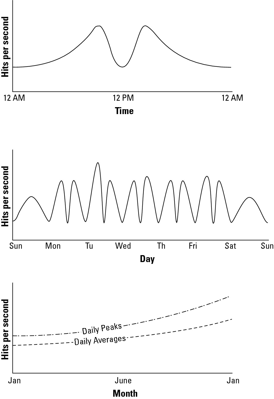
In Figure 6.1, the historical record for the Web server page views over a hypothetical day, week, and year are graphed. These graphs are created by summing the data from the different servers contained in the performance Web logs of the site or measuring throughput from the system based on an intervening service (such as a proxy server). What Figure 6.1 shows is a measure of the overall workload of the Web site involved.

Tip

Your performance logs are a primary source of data that everyone should have available for planning purposes, but they are not the only source of performance measurements. A number of companies offer services that can monitor your Web service's performance. For example, sites such as Alertra (http://www.alertra.com), Keynote (http://www.keynote.com), Gomez (http://www.gomez.com), PingDom (http://www.pingdom.com), and SiteUpTime (http://www.siteuptime.com) can monitor your Web pages to determine their response, latency, uptime, and other characteristics. Gomez and Keynote expose your site data visually as a set of dashboard widgets. Because these are third-party services, many Web services use these sites as the compliance monitor for Service Level Agreements (SLAs).

Notice several things about the graphs in Figure 6.1. A typical daily log (shown on top) shows two spikes in demand, one that is centered around 10 AM EST when users on the east coast of the United States use the site heavily and another at around 1 PM EST (three hours later; 10 AM PST) when users on the west coast of the United States use the site heavily. The three-hour time difference is also the difference between Eastern Standard Time and Pacific Standard Time.

These daily performance spikes occur on workdays, but the spikes aren't always of equal demand, as you can see from the weekly graph, shown in the middle of Figure 6.1. On weekends (Saturday and Sunday), the demand rises through the middle of the day and then ebbs later. Some days show a performance spike, as shown on the Tuesday morning section of the weekly graph. A goal of capacity planning (and an important business goal) is to correlate these performance spikes and dips with particular events and causations. Also, at some point your traffic patterns may change, so you definitely want to evaluate these statistics on an ongoing basis.

The yearly graph, at the bottom of Figure 6.1, shows that the daily averages and the daily peaks rise steadily over the year and, in fact, double from January 1st at the start of the year to December 31st at year end. Knowing this, a capacity planner would need to plan to serve twice the traffic while balancing the demands of peak versus average loads. However, it may not mean that twice the resources need to be deployed. The amount of resources to be deployed depends upon the characterization of the Web servers involved, their potential utilization rates, and other factors.

Caution

In predicting trends, it is important that the time scale be selected appropriately. A steady sure rise in demand over a year is much more accurate in predicting future capacity requirements than a sharp spike over a day or a week. Forecasting based on small datasets is notoriously inaccurate. You can't accurately predict the future (no one can), but you can make good guesses based on your intuition.

The total workload might be served by a single server instance in the cloud, a number of virtual server instances, or some combination of physical and virtual servers.

FIGURE 6.1

A Web servers' workload measured on a day, a week, and over the course of a year

A number of important characteristics are determined by these baseline studies:

• WT, the total workload for the system per unit time

To obtain WT, you need to integrate the area under the curve for the time period of interest.

• WAVG, the average workload over multiple units of time

To obtain WAVG, you need to sum various WTs and divide by the number of unit times involved. You may also want to draw a curve that represents the mean work done.

• WMAX, the highest amount of work recorded by the system

This is the highest recorded system utilization. In the middle graph of Figure 6.1, it would be the maximum number recorded on Tuesday morning.

• WTOT, the total amount of work done by the system, which is determined by the sum of WT (ΣWT)

A similar set of graphs would be collected to characterize the database servers, with the workload for those servers measured in transactions per second. As part of the capacity planning exercise, the workload for the Web servers would be correlated with the workload of the database servers to determine patterns of usage.

The goal of a capacity planning exercise is to accommodate spikes in demand as well as the overall growth of demand over time. Of these two factors, the growth in demand over time is the most important consideration because it represents the ability of a business to grow. A spike in demand may or may not be important enough to an activity to attempt to capture the full demand that the spike represents.

System metrics

Notice that in the previous section, you determined what amounts to application-level statistics for your site. These measurements are an aggregate of one or more Web servers in your infrastructure. Capacity planning must measure system-level statistics, determining what each system is capable of, and how resources of a system affect system-level performance.

In some instances, the capacity planner may have some influence on system architecture, and the impact of system architecture on application- and system-level statistics may be examined and altered. Because this is a rare case, let's focus on the next step, which defines system performance.

A machine instance (physical or virtual) is primarily defined by four essential resources:

• CPU

• Memory (RAM)

• Disk

• Network connectivity

Each of these resources can be measured by tools that are operating-system-specific, but for which tools that are their counterparts exist for all operating systems. Indeed, many of these tools were written specifically to build the operating systems themselves, but that's another story. In Linux/UNIX, you might use the sar command to display the level of CPU activity. sar is installed in Linux as part of the sysstat package. In Windows, a similar measurement may be made using the Task Manager, the data from which can be dumped to a performance log and/or graphed.

Some tools give you a historical record of performance, which is particularly useful in capacity planning. For example, the popular Linux performance measurement tool RRDTool (the Round Robin Database tool; http://oss.oetiker.ch/rrdtool/) is valuable in this regard. RRDTool is a utility that can capture time-dependent performance data from resources such as a CPU load, network utilization (bandwidth), and so on and store the data in a circular buffer. It is commonly used in performance analysis work.

A time interval in RRDTool is called a step, with the value in a step referred to as a primary data point (PDP). When a function is applied to a data point (average, minimum, maximum, and so on), the function is referred to as a Consolidation Function (CF), and the value obtained is a Consolidated Data Point (CDP). An interval is stored in the Round Robin Archive (RRA), and when that interval is filled, it is replaced by new step data. RRDToolincludes a graphical front end for displaying performance results visually. RRDTool is widely used for a number of different purposes. Figure 6.2 shows some of the examples from a gallery of RRDTool graphs found at http://oss.oetiker.ch/rrdtool/gallery/.

FIGURE 6.2

RRDTool lets you create historical graphs of a wide variety of performance data. Some samples are shown in the gallery at http://oss.oetiker.ch/rrdtool/gallery/.

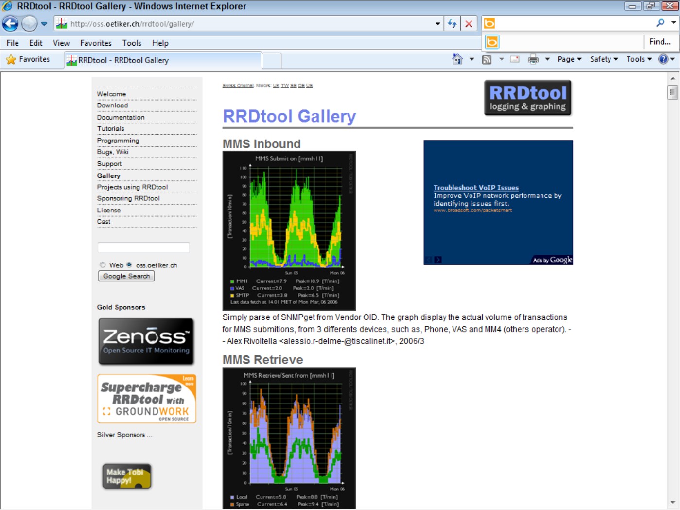
Table 6.1 lists some LAMP performance testing tools.

Load testing

Examining your server under load for system metrics isn't going to give you enough information to do meaningful capacity planning. You need to know what happens to a system when the load increases. Load testing seeks to answer the following questions:

1. What is the maximum load that my current system can support?

2. Which resource(s) represents the bottleneck in the current system that limits the system's performance?

This parameter is referred to as the resource ceiling. Depending upon a server's configuration, any resource can have a bottleneck removed, and the resource ceiling then passes onto another resource.

3. Can I alter the configuration of my server in order to increase capacity?

4. How does this server's performance relate to your other servers that might have different characteristics?

Note

Load testing is also referred to as performance testing, reliability testing, stress testing, and volume testing.

If you have one production system running in the cloud, then overloading that system until it breaks isn't going to make you popular with your colleagues. However, cloud computing offers virtual solutions. One possibility is to create a clone of your single system and then use a tool to feed that clone a recorded set of transactions that represent your application workload.

Two examples of applications that can replay requests to Web servers are HTTPerf (http://hpl.hp.com/research/linux/httperf/) and Siege (http://www.joedog.org/JoeDog/Siege), but both of these tools run the requests from a single client, which can be a resource limitation of its own. You can run Autobench (http://www.xenoclast.org/autobench/) to run HTTPerf from multiple clients against your Web server, which is a better test.

You may want to consider these load generation tools as well:

• HP LodeRunner (https://h10078.www1.hp.com/cda/hpms/display/main/hpms_content.jsp?zn=bto&cp=1-11-126-17^8_4000_100__)

• IBM Rational Performance Tester (http://www-01.ibm.com/software/awdtools/tester/performance/)

• JMeter (http://jakarta.apache.org/jmeter)

• OpenSTA (http://opensta.org/)

• Micro Focus (Borland) SilkPerfomer (http://www.borland.com/us/products/silk/silkperformer/index.html)

Load testing software is a large product category with software and hardware products. You will find load testing useful in testing the performance of not only Web servers, but also application servers, database servers, network throughput, load balancing servers, and applications that rely on client-side processing.

When you have multiple virtual servers that are part of a server farm and have a load balancer in front of them, you can use your load balancer to test your servers' resource ceilings. This technique has the dual advantages of allowing you to slowly increment traffic on a server and to use real requests while doing so. Most load balancers allow you to weight the requests going to a specific server with the goal of serving more requests to more powerful systems and fewer requests to less powerful systems. Sometimes the load balancer does this optimization automatically, and other times you can exert manual control over the weighting.

Whatever method you use to load a server for performance testing, you must pick a method that is truly representative of real events, requests, and operations. The best approach is to incrementally alter the load on a server with the current workload. When you make assumptions such as using a load balancer to serve traffic based on a condition that summarizes the traffic pattern instead of using the traffic itself, you can get yourself into trouble.

Problems with load balancers have led to some spectacular system failures because those devices occupy a central controlling site in any infrastructure. For example, if you assume that traffic can be routed based on the number of connections in use per server and your traffic places a highly variable load based on individual requests, then your loading measurements can lead to dramatic failures when you attempt to alter your infrastructure to accommodate additional loads.

Resource ceilings

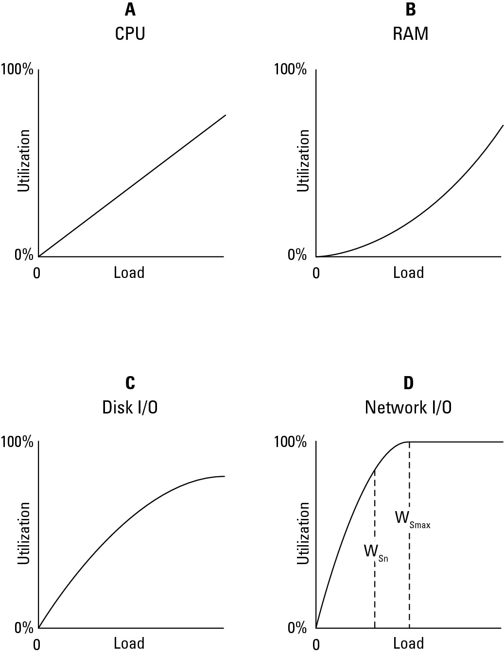
Whatever performance measurement tool you use, the goal is to create a set of resource utilization curves similar to the ones shown in Figure 6.3 for individual server types in your infrastructure. To do this, you must examine the server at different load levels and measure utilization rates.

The graphs in Figure 6.3 indicate that over a certain load for a particular server, the CPU (A), RAM (B), and Disk I/O (C) utilization rates rise but do not reach their resource ceiling. In this instance, the Network I/O (D) reaches its maximum 100-percent utilization at about 50 percent of the tested load, and this factor is the current system resource ceiling.

Network I/O is often a bottleneck in Web servers, and this is why, architecturally, Web sites prefer to scale out using many low-powered servers instead of scaling up with fewer but more powerful servers. You saw this play out in the previous chapter where Google's cloud was described. Adding more (multi-homing) or faster network connections can be another solution to improving Web servers' performance.

Unless you alter the performance of the server profiled in Figure 6.3 to improve it, you are looking at a maximum value for that server's workload of WSmax, as shown in the dashed line at the 50-percent load point in graph D. At this point, the server is overloaded and the system begins to fail. Some amount of failure may be tolerable in the short term, provided that the system can recover and not too many Web hits are lost, but this is a situation that you really want to minimize. You can consider WSn to be the server's red line, the point at which the system should be generating alerts or initiating scripts to increase capacity.

FIGURE 6.3

Resource utilization curves for a particular server

Notice that I have not discussed whether these are physical or virtual servers. The parameter you are most interested in is likely to be the overall system capacity, which is the value of WT.

WT is the sum over all the Web servers in your infrastructure:

WT = Σ(WSnP WSnV)

In this equation, WSnP represents the workload of your physical server(s) and WSnV is the workload of the virtual servers (cloud-based server instances) of your infrastructure. The amount of overhead you allow yourself should be dictated by the amount of time you require to react to the challenge and to your tolerance for risk. A capacity planner would define a value WT such that there is sufficient overhead remaining in the system to react to demand that is defined by a number greater than WMAX by bringing more resources on-line. For storage resources that tend to change slowly, a planner might set the red line level to be 85 percent of consumption of storage; for a Web server, that utilization percentage may be different. This setting would give you a 15-percent safety factor.

There are more factors that you might want to take into account when considering an analysis of where to draw the red line. When you load test a system, you are applying a certain amount of overhead to the system from the load testing tool—a feature that is often called the “observer effect.” Many load testers work by installing lightweight agents on the systems to be tested. Those agents themselves impact the performance you see; generally though, their impact is limited to a few percent. Additionally, in order to measure performance, you may be forced to turn on various performance counters. A performance counter is also an agent of sorts; the counter is running a routine that measures some aspect of performance such as queue length, file I/O rate, numbers of READs and WRITEs, and so forth. While these complications are second order effects, it's always good to keep this in mind and not over-interpret performance results.

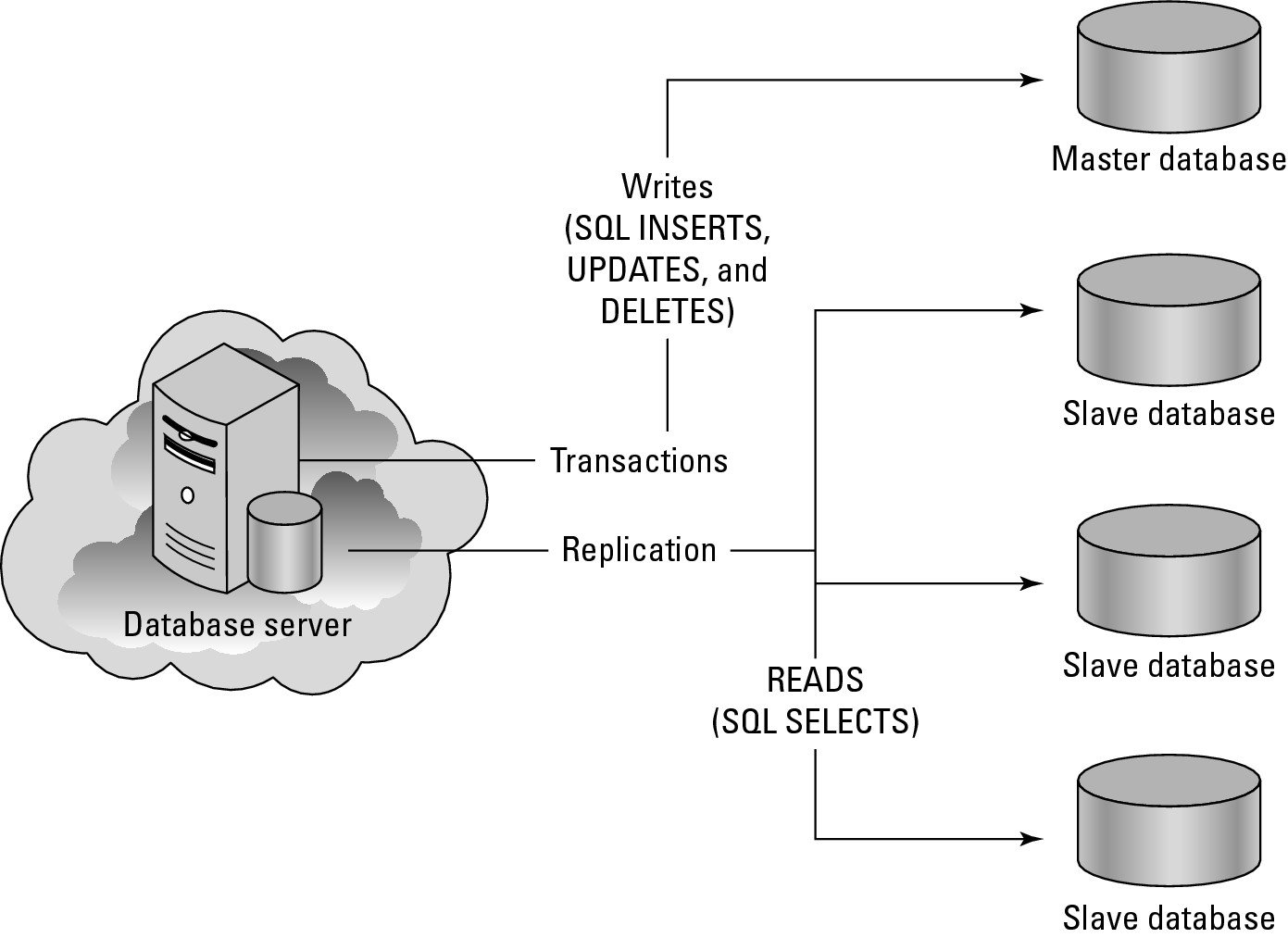
Before leaving the topic of resource ceilings, let's consider a slightly more complicated case that you might encounter in MySQL database systems. Database servers are known to exhibit resource ceilings for either their file caches or their Disk I/O performance. To build high-performance applications, many developers replicate their master MySQL database and create a number of slave MySQL databases. All READ operations are performed on the slave MySQL databases, and all WRITE operations are performed on the master MySQL database. Figure 6.4 shows this sort of database architecture.

A master/slave database system has two competing processes and the same server that are sharing a common resource: READs and WRITEs to the master/slave databases, and replication traffic between the master database and all the slave databases. The ratio of these transactions determines the WSn for the system, and the WSn you derive is highly dependent upon the system architecture. These types of servers reach failure when the amount of WRITEtraffic in the form of INSERT, UPDATE, and DELETE operations to the master database overtakes the ability of the system to replicate data to the slave databases that are servicing SELECT (query/READ) operations.

The more slave databases there are, the more actively the master database is being modified and the lower the WS for the master database is. This system may support no more than 25-35 percent transactional workload as part of its overall capacity, depending upon the nature of the database application you are running.

You increase the working capacity of a database server that has a Disk I/O resource ceiling by using more powerful disk arrays and improving the interconnection or network connection used to connect the server to its disks. Disk I/O is particularly sensitive to the number of spindles in use, so having more disks equals greater performance. Keep in mind that your ability to alter the performance of disk assets in a virtual or cloud-based database server is generally limited.

Tip

A master/slave MySQL replication architectural scheme is used for smaller database applications. As sites grow and the number of transactions increases, developers tend to deploy databases in a federated architecture. The description of Google's cloud in Chapter 5 describes this approach to large databases, creating what are called sharded databases.

FIGURE 6.4

Resource contention in a database server

So far you've seen two cases. In the first case, a single server has a single application with a single resource ceiling. In the second case, you have a single server that has a single application with two competing processes that establish a resource ceiling. What do you do in a situation where your server runs the full LAMP stack and you have two or more applications running processes each of which has its own resource ceiling? In this instance, you must isolate each application and process and evaluate their characteristics separately while trying to hold the other applications' resource usage at a constant level. You can do this by examining identical servers running the application individually or by creating a performance console that evaluates multiple factors all at the same time. Remember, real-world data and performance is always preferred over simulations.

As your infrastructure grows, it becomes more valuable to create a performance console that lets you evaluate your KPIs (Key Performance Indicators) graphically at an instant. Many third-party tools offer performance consoles, and some tools allow you to capture their state so you can restore it at a later point. An example of a performance analysis tool that lets you save its state is the Microsoft Management Console (MMC). In the Amazon Web Service, the statistics monitoring tool is called Amazon CloudWatch, and you can create a performance monitoring console from the statistics it collects.

Server and instance types

One goal of capacity planning is to make growth and shrinkage of capacity predictable. You can greatly improve your chances by standardizing on a few hardware types and then well characterizing those platforms. In a cloud infrastructure such as Amazon Web Server, the use of different machine instance sizes is an attempt to create standard servers. Reducing the variability between servers makes it easier to troubleshoot problems and simpler to deploy and configure new systems.

As much as possible, you also should assign servers standardized roles and populate those servers with identical services. A server with the same set of software, system configuration, and hardware should perform similarly if given the same role in an infrastructure. At least that's the theory.

In practice, cloud computing isn't quite as mature as many organizations' physical servers, and in practice, there is more performance variability in cloud machine instances than you might expect. This variability may be due to your machine instances or storage buckets being moved from one system to another system. Therefore, you should be attentive to the increase in potential for virtual system variability and build additional safety factors into your infrastructure. System instances in a cloud can fail, and it is up to the client to recognize these failures and react accordingly. Virtual machines in a cloud are something of a black box, and you should treat them as such because you have no idea what the underlying physical reality of the resources you are using represents.

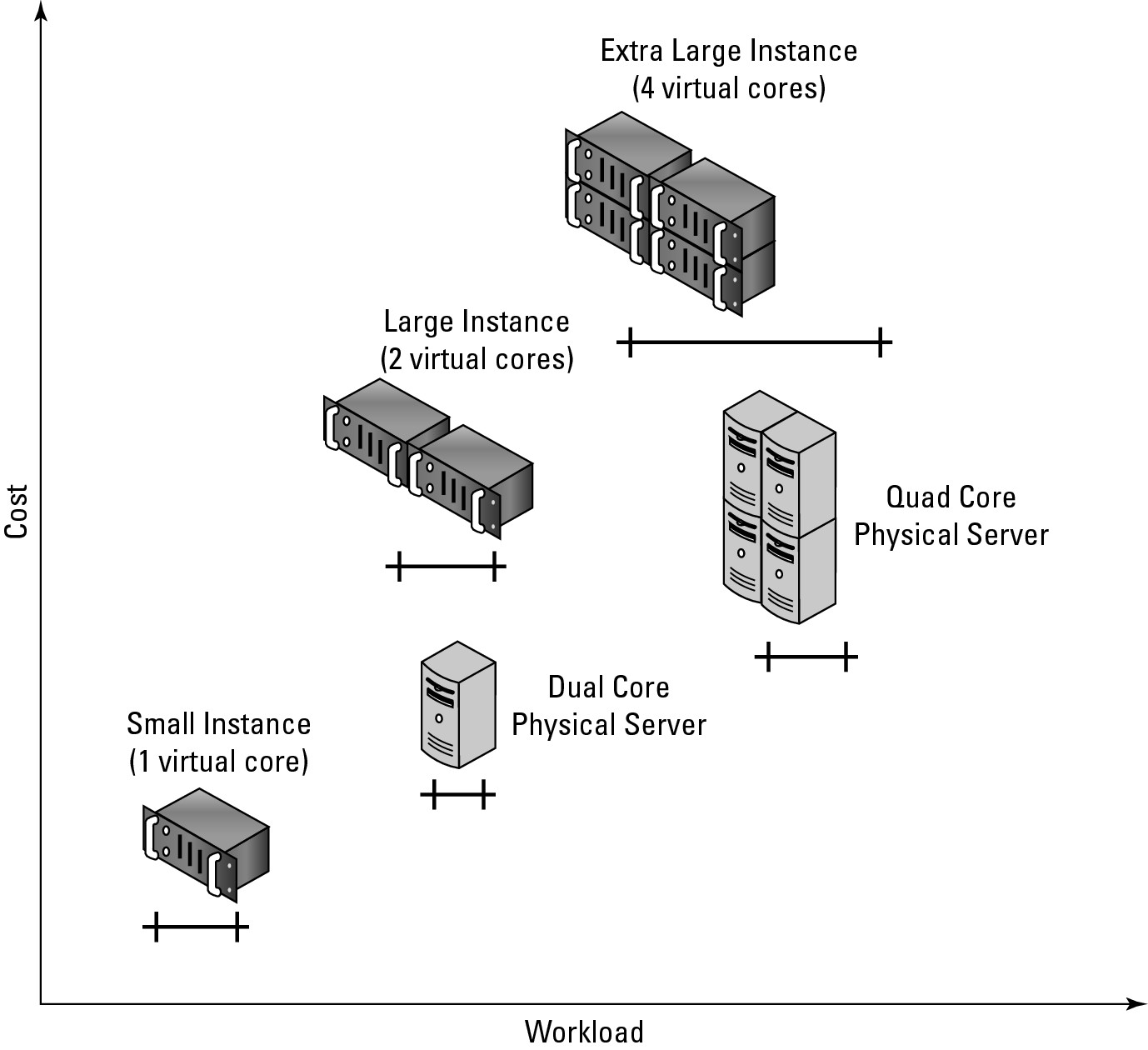
Capacity planning seeks to compare the capability of one system against another system and to choose the solution that is not only the right size but provides the service with the best operational parameters at the lowest cost. In Figure 6.5, a graph of different server types is shown, with some hypothetical physical servers plotted against Amazon Machine Instance types. This type of graph allows you to add the appropriate server type to your infrastructure while performing a cost analysis of the deployment.

An Amazon Machine Instance (AMI) is described as follows:

• Micro Instance: 633 MB memory, 1 to 2 EC2 Compute Units (1 virtual core, using 2 CUs for short periodic bursts) with either a 32-bit or 64-bit platform

• Small Instance (Default): 1.7GB memory, 1 EC2 Compute Unit (1 virtual core with 1 EC2 Compute Unit), 160GB instance storage (150GB plus 10GB root partition), 32-bit platform, I/O Performance: Moderate, and API name: m1.small

• High-Memory Quadruple Extra Large Instance: 68.4GB of memory, 26 EC2 Compute Units (8 virtual cores with 3.25 EC2 Compute Units each), 1,690GB of instance storage, 64-bit platform, I/O Performance: High, and API name: m2.4xlarge

• High-CPU Extra Large Instance: 7GB of memory, 20 EC2 Compute Units (8 virtual cores with 2.5 EC2 Compute Units each), 1,690GB of instance storage, 64-bit platform, I/O Performance: High, API name: c1.xlarge

View this at http://aws.amazon.com/ec2/instance-types/; I expand on this in Chapter 9.

FIGURE 6.5

Relative costs and efficiencies of different physical and virtual servers

While you may not know what exactly EC2 Compute Unit or I/O Performance High means, at least we can measure these performance claims and attach real numbers to them. Amazon says that an EC2 Compute Unit is the equivalent of a 1.0-1.2 GHz 2007 Opteron or 2007 Xeon processor, but adds that “Over time, we may add or substitute measures that go into the definition of an EC2 Compute Unit, if we find metrics that will give you a clearer picture of compute capacity.” What they are saying essentially is that this was the standard processor their fleet used as its baseline, and that over time more powerful systems may be swapped in. Whatever the reality of this situation, from the standpoint of capacity planning, all you should care about is measuring the current performance of systems and right-sizing your provisioning to suit your needs.

In cloud computing, you can often increase capacity on demand quickly and efficiently. Not all cloud computing infrastructures automatically manage your capacity for you as Amazon Web Service's Auto Scaling (http://aws.amazon.com/autoscaling/) feature does. At this point in the maturity of the industry, some systems provide automated capacity adjustments, but most do not.

Nor are you guaranteed to be provided with the needed resources from a cloud vendor at times you might need it most. For example, Amazon Web Services' infrastructure runs not only clients' machine instances, but also Amazon.com's machine instances as well as Amazon.com's partners' instances. If you need more virtual servers on Black Monday to service Web sales, you may be out of luck unless you have an SLA that guarantees you the additional capacity. Finding an SLA that you can rely on is still something of a crap shoot. If you are in the position of having to maintain the integrity of your data for legal reasons, this imposes additional problems and constraints.

Cloud computing is enticing. It is easy to get started and requires little up-front costs. However, cloud computing is not cheap. As your needs scale, so do your costs, and you have to pay particular attention to costs as you go forward. At the point where you have a large cloud-based infrastructure, you may find that it is more expensive to have a metered per-use cost than to own your own systems. The efficiencies of cloud computing, as I describe more fully in Chapter 2, aren't necessarily in the infrastructure itself. Most of the long-term efficiencies are realized in the reduced need for IT staff and management, the ability to react quickly to business opportunities, and the freeing of a business from managing networked computer systems to concentrate on their core businesses. So while the Total Cost of Ownership (TCO) of a cloud-based infrastructure might be beneficial, it might be difficult to convince the people paying the bills that this is really so.

Network Capacity

If any cloud-computing system resource is difficult to plan for, it is network capacity. There are three aspects to assessing network capacity:

• Network traffic to and from the network interface at the server, be it a physical or virtual interface or server

• Network traffic from the cloud to the network interface

• Network traffic from the cloud through your ISP to your local network interface (your computer)

This makes analysis complicated. You can measure factor 1, the network I/O at the server's interface with system utilities, as you would any other server resource. For a cloud-based virtual computer, the network interface may be a highly variable resource as the cloud vendor moves virtual systems around on physical systems or reconfigures its network pathways on the fly to accommodate demand. But at least it is measurable in real time.

To measure network traffic at a server's network interface, you need to employ what is commonly known as a network monitor, which is a form of packet analyzer. Microsoft includes a utility called the Microsoft Network Monitor as part of its server utilities, and there are many third-party products in this area. The site Sectools.org has a list of packet sniffers at http://sectools.org/sniffers.html. Here are some:

• Wireshark (http://www.wireshark.org/), formerly called Ethereal

• Kismet (http://www.kismetwireless.net/), a WiFi sniffer

• TCPdump (http://www.tcpdump.org/)

• Dsniff (http://www.monkey.org/~dugsong/dsniff/)

• Ntop (http://www.ntop.org/)

• EtherApe (http://etherape.sourceforge.net/)

Regardless of which of these tools you use, the statistics function of these tools provides a measurement of network capacity as expressed by throughput. You can analyze the data in a number of ways, including specific applications used, network protocols, traffic by system or users, and so forth all the way down to, in some cases, the content of the individual packets crossing the wire.

Note

Alternative names for packet analyzer include network analyzer, network traffic monitor, protocol analyzer, packet sniffer, and Ethernet sniffer, and for wireless networks, wireless or wifi sniffer, network detector, and so on. To see a comparison chart of packet analyzers on Wikipedia, go to http://en.wikipedia.org/wiki/Comparison_of_packet_analyzers.

Factor 2 is the cloud's network performance, which is a measurement of WAN traffic. A WAN's capacity is a function of many factors:

• Overall system traffic (competing services)

• Routing and switching protocols

• Traffic types (transfer protocols)

• Network interconnect technologies (wiring)

• The amount of bandwidth that the cloud vendor purchased from an Internet backbone provider

Again, factor 2 is highly variable and unlike factor 1, it isn't easy to measure in a reliable way.

Tools are available that can monitor a cloud network's performance at geographical different points and over different third-party ISP connections. This is done by establishing measurement systems at various well-chosen network hubs.

Apparent Networks, a company that makes WAN network monitoring software, has set up a series of these points of presence at various Internet hubs and uses its networking monitoring software called PathView Cloud to collect data in a display that it calls the Cloud Performance Scorecard (http://www.apparentnetworks.com/CPC/scorecard.aspx). Figure 6.6 shows this Web page populated with statistics for some of the cloud vendors that Apparent Networks monitors. You can use PathView Cloud as a hosted service to evaluate your own cloud application's network performance at these various points of presence and to create your own scorecard of a cloud network. Current pricing for the service is $5 per network path per month. The company also sells a small appliance that you can insert at locations of your choice and with which you can perform your own network monitoring.

The last factor, factor 3, is the connection from the backbone through your ISP to your local system, a.k.a. “The Internet.” The “Internet” is not a big, fat, dumb pipe; nor is it (as former Senator Ted Stevens of Alaska proclaimed) “a series of tubes.” For most people, their Internet connection is more like an intelligently managed thin straw that you are desperately trying to suck information out of. So factor 3 is measurable, even if the result of the measurement isn't very encouraging, especially to your wallet.

Internet connectivity over the last mile (to the home) is the Achilles heel of cloud computing. The scarcity of high-speed broadband connections (particularly in the United States) and high pricing are major impediments to the growth of cloud computing. Many organizations and communities will wait on the sidelines before embracing cloud computing until faster broadband becomes available. Indeed, this may be the final barrier to cloud computing's dominance.

That's one of the reasons that large cloud providers like Google are interested in building their own infrastructure, in promoting high-speed broadband connectivity, and in demonstrating the potential of high-speed WANs. Google is running a demonstration project called Google Fibre for Communities (http://www.google.com/appserve/fiberrfi/public/overview) that will deliver 1 gigabit-per-second fiber to the home. The few lucky municipalities chosen (with 50,000 to 500,000 residents) for the demonstration project will get advanced broadband applications, many of which will be cloud-based. The winners of this contest have yet to be announced, but they are certain to be highly sought after (see Figure 6.7).

FIGURE 6.6

Apparent Networks' Cloud Performance Center provides data on WAN throughput and uptime at Internet network hubs.

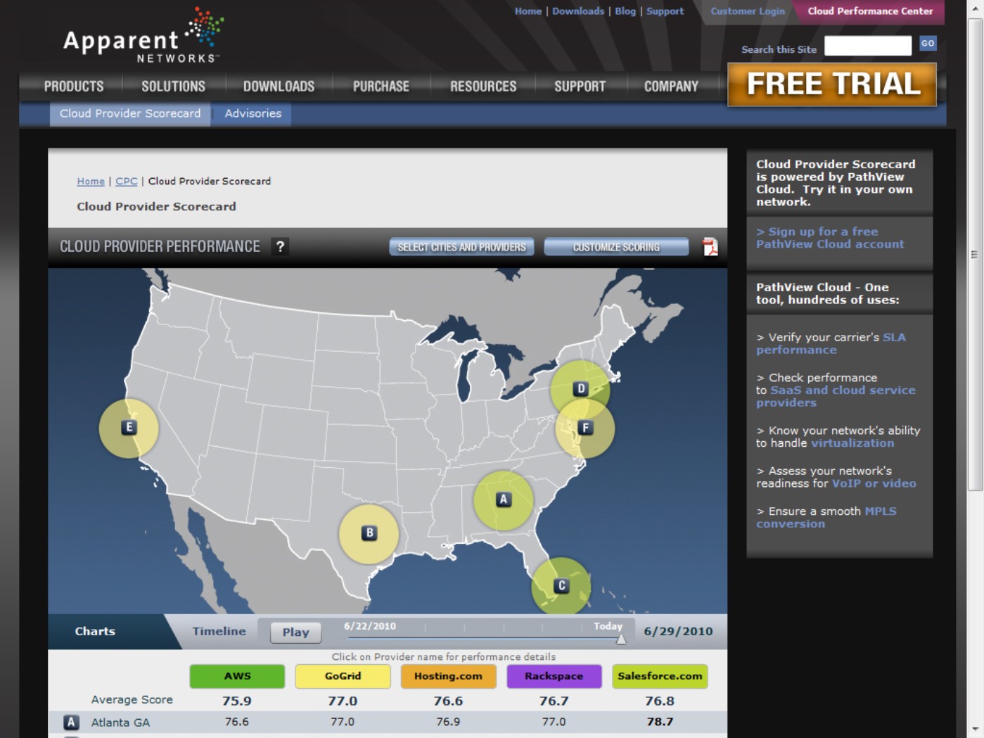
FIGURE 6.7

You are not in Kansas anymore. To petition Google for a Fiber for Communities network, Topeka, Kansas, became Google for a day, and Google returned the favor.

Scaling

In capacity planning, after you have made the decision that you need more resources, you are faced with the fundamental choice of scaling your systems. You can either scale vertically (scale up) or scale horizontally (scale out), and each method is broadly suitable for different types of applications.

To scale vertically, you add resources to a system to make it more powerful. For example, during scaling up, you might replace a node in a cloud-based system that has a dual-processor machine instance equivalence with a quad-processor machine instance equivalence. You also can scale up when you add more memory, more network throughput, and other resources to a single node. Scaling out indefinitely eventually leads you to an architecture with a single powerful supercomputer.

Vertical scaling allows you to use a virtual system to run more virtual machines (operating system instance), run more daemons on the same machine instance, or take advantage of more RAM (memory) and faster compute times. Applications that benefit from being scaled up vertically include those applications that are processor-limited such as rendering or memory-limited such as certain database operations—queries against an in-memory index, for example.

Horizontal scaling or scale out adds capacity to a system by adding more individual nodes. In a system where you have a dual-processor machine instance, you would scale out by adding more dual-processor machines instances or some other type of commodity system. Scaling out indefinitely leads you to an architecture with a large number of servers (a server farm), which is the model that many cloud and grid computer networks use.

Horizontal scaling allows you to run distributed applications more efficiently and is effective in using hardware more efficiently because it is both easier to pool resources and to partition them. Although your intuition might lead you to believe otherwise, the world's most powerful computers are currently built using clusters of computers aggregated using high speed interconnect technologies such as InfiniBand or Myrinet. Scale out is most effective when you have an I/O resource ceiling and you can eliminate the communications bottleneck by adding more channels. Web server connections are a classic example of this situation.

These broad generalizations between scale up and scale out are useful from a conceptual standpoint, but the reality is that there are always tradeoffs between choosing one method for scaling your cloud computing system versus the other. Often, the choice isn't so clear-cut. The pricing model that cloud computing vendors now offer their clients isn't fully mature at the moment, and you may find yourself paying much more for a high-memory extra-large machine instance than you might pay for the equivalent amount of processing power purchased with smaller system equivalents. This has always been true when you purchase physical servers, and it is still true (but to a much smaller extent) when purchasing virtual servers. Cost is one factor to pay particular attention to, but there are other tradeoffs as well. Scale out increases the number of systems you must manage, increases the amount of communication between systems that is going on, and introduces additional latency to your system.

Summary

In this chapter, you learned about how to match capacity to demand. To do this, you must measure performance of your systems, predict demand, and understand demand patterns. You must them allocate resources to meet demands. When demand is higher, you must provision additional resources, and when demand is lower, you must tear down resources currently in place.

Cloud computing's use of virtual resources offers exciting new ways to flexibly respond to demand challenges. Cloud computing also poses some new risks and makes additional demands on the capacity planner that this chapter discusses.

The key to capacity planning is through measurement of current system performance and the collection of a meaningful historical data set. This chapter described some of the tools you need to perform these analyses, a general approach you must take, and how to act based on the results you find.

In Chapter 7, I more fully explore the Platform as a Service (PaaS) model that provides a new application delivery paradigm. PaaS is the delivery of a complete computer platform as well as an application stack. You can use systems of these types to create solutions that you use or offer to others as a service. Because the infrastructure and architecture is already in place, PaaS allows you to concentrate on a very specific service that leverages the investment already made by the PaaS vendor. Chapter 7 describes some of these types of services, the application frameworks used in PaaS, and some of the programming tools in place.