Algorithms Third Edition in C++ Part 5. Graph Algorithms (2006)
CHAPTER EIGHTEEN
Graph Search
18.6 Separability and Biconnectivity
To illustrate the power of DFS as the basis for graph-processing algorithms, we turn to problems related to generalized notions of connectivity in graphs. We study questions such as the following: Given two vertices, are there two different paths connecting them?
If it is important that a graph be connected in some situation, it might also be important that it stay connected when an edge or a vertex is removed. That is, we may want to have more than one route between each pair of vertices in a graph, so as to handle possible failures. For example, we can fly from New York to San Francisco even if Chicago is snowed in by going through Denver instead. Or, we might imagine a wartime situation where we want to arrange our railroad network such that an enemy must destroy at least two stations to cut our rail lines. Similarly, we might expect the main communications lines in an integrated circuit or a communications network to be connected such that the rest of the circuit still can function if one wire is broken or one link is down.
These examples illustrate two distinct concepts: In the circuit and in the communications network, we are interested in staying connected if an edge is removed; in the air or train routes, we are interested in staying connected if a vertex is removed. We begin by examining the former in detail.
Figure 18.16 An edge-separable graph
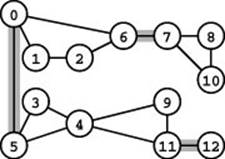
This graph is not edge connected. The edges 0-5, 6-7, and 11-12 (shaded) are separating edges (bridges). The graph has 4 edge-connected components: one comprising vertices 0, 1, 2, and 6; another comprising vertices 3, 4, 9, and 11; another comprising vertices 7, 8, and 10; and the single vertex 12.
Definition 18.1 A bridge in a graph is an edge that, if removed, would separate a connected graph into two disjoint subgraphs. A graph that has no bridges is said to be edge-connected.
When we speak of removing an edge, we mean to delete that edge from the set of edges that define the graph, even when that action might leave one or both of the edge’s vertices isolated. An edge-connected graph remains connected when we remove any single edge. In some contexts, it is more natural to emphasize our ability to disconnect the graph rather than the graph’s ability to stay connected, so we freely use alternate terminology that provides this emphasis: We refer to a graph that is not edge-connected as an edge-separable graph, and we call bridges separation edges. If we remove all the bridges in an edge-separable graph, we divide it into edge-connected components or bridge-connected components: maximal subgraphs with no bridges. Figure 18.16 is a small example that illustrates these concepts.
Finding the bridges in a graph seems, at first blush, to be a nontrivial graph-processing problem, but it actually is an application of DFS where we can exploit basic properties of the DFS tree that we have already noted. Specifically, back edges cannot be bridges because we know that the two nodes they connect are also connected by a path in the DFS tree. Moreover, we can add a simple test to our recursive DFS function to test whether or not tree edges are bridges. The basic idea, stated formally next, is illustrated in Figure 18.17.
Property 18.5 In any DFS tree, a tree edge v-w is a bridge if and only if there are no back edges that connect a descendant of w to an ancestor of w .
Proof: If there is such an edge, v-w cannot be a bridge. Conversely, if v-w is not a bridge, then there has to be some path from w to v in the graph other than w-v itself. Every such path has to have some such edge. •
Asserting this property is equivalent to saying that the only link in the subtree rooted at w that points to a node not in the subtree is the parent link from w back to v. This condition holds if and only if every path connecting any of the nodes in w’s subtree to any node that
Figure 18.17 DFS tree for finding bridges
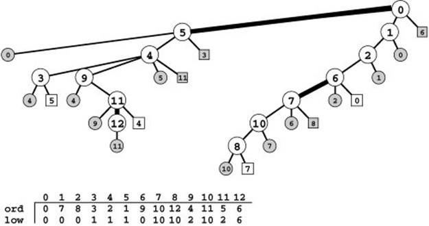
Nodes 5, 7, and 12 in this DFS tree for the graph in Figure 18.16 all have the property that no back edge connects a descendant with an ancestor, and no other nodes have that property. Therefore, as indicated, breaking the edge between one of these nodes and its parent would disconnect the subtree rooted at that node from the rest of the graph. That is, the edges 0-5, 11-12, and 6-7 are bridges. We use the vertex-indexed array low to keep track of the lowest preorder number (ord value) referenced by any back edge in the subtree rooted at the vertex. For example, the value of low[9] is 2 because one of the back edges in the subtree rooted at 9 points to 4 (the vertex with preorder number 2), and no other back edge points higher in the tree. Nodes 5, 7, and 12 are the ones for which the low value is equal to the ord value.
is not in w’s subtree includes v-w. In other words, removing v-w would disconnect from the rest of the graph the subgraph corresponding to w’s subtree.
Program 18.7 shows how we can augment DFS to identify bridges in a graph, using Property 18.5. For every vertex v, we use the recursive function to compute the lowest preorder number that can be reached by a sequence of zero or more tree edges followed by a single back edge from any node in the subtree rooted at v. If the computed number is equal to v’s preorder number, then there is no edge connecting a descendant with an ancestor, and we have identified a bridge. The computation for each vertex is straightforward: We proceed through the adjacency list, keeping track of the minimum of the numbers that we can reach by following each edge. For tree edges, we do the computation recursively; for back edges, we use the preorder number of the adjacent vertex. If the call to the recursive function for an edge w-t does not uncover a path to a node with a preorder number less than t’s preorder number, then w-t is a bridge.
Property 18.6 We can find a graph’s bridges in linear time.
Proof: Program 18.7 is a minor modification to DFS that involves adding a few constant-time tests, so it follows directly from Properties 18.3 and 18.4 that finding the bridges in a graph requires time proportional to V2 for the adjacency-matrix representation and to V + E for the adjacency-lists representation.•
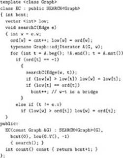
Program 18.7 Edge connectivity
This DFS class counts the bridges in a graph. Clients can use an EC object to find the number of edge-connected components; adding a member function for testing whether two vertices are in the same edge-connected component is left as an exercise (see Exercise 18.36). The low vector keeps track of the lowest preorder number that can be reached from each vertex by a sequence of tree edges followed by one back edge.
In Program 18.7, we use DFS to discover properties of the graph. The graph representation certainly affects the order of the search, but it does not affect the results because bridges are a characteristic of the graph rather than of the way that we choose to represent or search
Figure 18.18 Another DFS tree for finding bridges
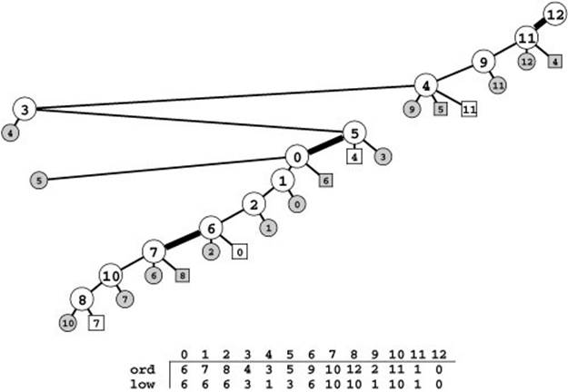
This diagram shows a different DFS tree than the one in Figure 18.17 for the graph in Figure 18.16, where we start the search at a different node. Although we visit the nodes and edges in a completely different order, we still find the same bridges (of course). In this tree, 0, 7, and 11 are the ones for which the low value is equal to the ord value, so the edges connecting each of them to their parents (12-11, 5-0, and 6-7, respectively) are bridges.
the graph. As usual, any DFS tree is simply another representation of the graph, so all DFS trees have the same connectivity properties. The correctness of the algorithm depends on this fundamental fact. For example, Figure 18.18 illustrates a different search of the graph, starting from a different vertex, that (of course) finds the same bridges. Despite Property 18.6, when we examine different DFS trees for the same graph, we see that some search costs may depend not just on properties of the graph but also on properties of the DFS tree. For example, the amount of space needed for the stack to support the recursive calls is larger for the example in Figure 18.18 than for the example in Figure 18.17.
As we did for regular connectivity in Program 18.4, wemaywish to use Program 18.7 to build a class for testing whether a graph is edge-connected or to count the number of edge-connected components. If desired, we can proceed as for Program 18.4 to gives clients the ability to create (in linear time) objects that can respond in constant time to queries that ask whether two vertices are in the same edge-connected component (see Exercise 18.36).
We conclude this section by considering other generalizations of connectivity, including the problem of determining which vertices are critical to keeping a graph connected. By including this material here, we keep in one place the basic background material for the more complex algorithms that we consider in Chapter 22. If you are new to connectivity problems, you may wish to skip to Section 18.7 and return here when you study Chapter 22.
When we speak of removing a vertex, we also mean that we remove all its incident edges. As illustrated in Figure 18.19, removing either of the vertices on a bridge would disconnect a graph (unless the bridge were the only edge incident on one or both of the vertices), but there are also other vertices, not associated with bridges, that have the same property.
Definition 18.2 An articulation point in a graph is a vertex that, if removed, would separate a connected graph into at least two disjoint subgraphs.
We also refer to articulation points as separation vertices or cut vertices. We might use the term “vertex connected” to describe a graph that has no separation vertices, but we use different terminology based on a related characterization that turns out to be equivalent.
Definition 18.3 A graph is said to be biconnected if every pair of vertices is connected by two disjoint paths.
The requirement that the paths be disjoint is what distinguishes biconnectivity from edge connectivity. An alternate definition of edge connectivity is that every pair of vertices is connected by two edge-disjoint paths—these paths can have a vertex (but no edge) in common. Biconnectivity is a stronger condition: An edge-connected graph remains connected if we remove any edge, but a biconnected graph remains connected if we remove any vertex (and all that vertex’s incident edges). Every biconnected graph is edge-connected, but an edge-connected graph need not be biconnected. We also use the term separable to refer to graphs that are not biconnected, because they can be separated into two pieces by removal of just one vertex. The separation vertices are the key to biconnectivity.
Property 18.7 A graph is biconnected if and only if it has no separation vertices (articulation points).
Proof: Assume that a graph has a separation vertex. Let s and t be vertices that would be in two different pieces if the separation vertex were removed. All paths between s and t must contain the separation vertex, therefore the graph is not biconnected. The proof in the other direction is more difficult and is a worthwhile exercise for the mathematically inclined reader (see Exercise 18.40).•
Figure 18.19 Graph separability terminology
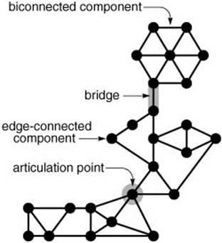
This graph has two edge-connected components and one bridge. The edge-connected component above the bridge is also biconnected; the one below the bridge consists of two biconnected components that are joined at an articulation point.
Figure 18.20 Articulation points (separation vertices)
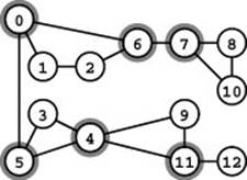
This graph is not biconnected. The vertices 0, 4, 5, 6, 7, and 11 (shaded) are articulation points. The graph has five biconnected components: one comprising edges 4-9, 9-11, and 4-11; another comprising edges 7-8, 8-10, and 7-10; another comprising edges 0-1, 1-2, 2-6, and 6-0; another comprising edges 3-5, 4-5, and 3-4; and the single vertex 12. Adding an edge connecting 12 to 7, 8, or 10 would biconnect the graph.
We have seen that we can partition the edges of a graph that is not connected into a set of connected subgraphs, and that we can partition the edges of a graph that is not edge-connected into a set of bridges and edge-connected subgraphs (which are connected by bridges). Similarly, we can divide any graph that is not biconnected into a set of bridges and biconnected components, which are each biconnected subgraphs. The biconnected components and bridges are not a proper partition of the graph because articulation points may appear on multiple biconnected components (see, for example, Figure 18.20). The biconnected components are connected at articulation points, perhaps by bridges.
A connected component of a graph has the property that there exists a path between any two vertices in the graph. Analogously, a biconnected component has the property that there exist two disjoint paths between any pair of vertices.
We can use the same DFS-based approach that we used in Program 18.7 to determine whether or not a graph is biconnected and to identify the articulation points. We omit the code because it is very similar to Program 18.7, with an extra test to check whether the root of the DFS tree is an articulation point (see Exercise 18.43). Developing code to print out the biconnected components is also a worthwhile exercise that is only slightly more difficult than the corresponding code for edge connectivity (see Exercise 18.44).
Property 18.8 We can find a graph’s articulation points and biconnected components in linear time.
Proof: As for Property 18.7, this fact follows from the observation that the solutions to Exercises 18.43 and 18.44 involve minor modifications to DFS that amount to adding a few constant-time tests per edge.
Biconnectivity generalizes simple connectivity. Further generalizations have been the subjects of extensive studies in classical graph theory and in the design of graph algorithms. These generalizations indicate the scope of graph-processing problems that we might face, many of which are easily posed but less easily solved.
Definition 18.4 Agraphis k-connected if there are at least k vertex-disjoint paths connecting every pair of vertices in the graph. The vertex connectivity of a graph is the minimum number of vertices that need to be removed to separate it into two pieces.
In this terminology, “1-connected” is the same as “connected” and “2-connected” is the same as “biconnected.” A graph with an articulation point has vertex connectivity 1 (or 0), so Property 18.7 says that a graph is 2-connected if and only if its vertex connectivity is not less than 2. It is a special case of a classical result from graph theory, known as Whitney’s theorem, which says that a graph is k -connected if and only if its vertex connectivity is not less than k. Whitney’s theorem follows directly from Menger’s theorem (see Section 22.7), which says that the minimum number of vertices whose removal disconnects two vertices in a graph is equal to the maximum number of vertex-disjoint paths between the two vertices (to prove Whitney’s theorem, apply Menger’s theorem to every pair of vertices).
Definition 18.5 A graph is k–edge-connected if there are at least k edge-disjoint paths connecting every pair of vertices in the graph. The edge connectivity of a graph is the minimum number of edges that need to be removed to separate it into two pieces.
In this terminology, “2–edge-connected” is the same as “edge-connected” (that is, an edge-connected graph has edge connectivity greater than 1, and a graph with at least one bridge has edge connectivity 1). Another version of Menger’s theorem says that the minimum number of vertices whose removal disconnects two vertices in a graph is equal to the maximum number of vertex-disjoint paths between the two vertices, which implies that a graph is k –edge-connected if and only if its edge connectivity is k.
With these definitions, we are led to generalize the connectivity problems that we considered at the beginning of this section.
st-connectivity What is the minimum number of edges whose removal will separate two given vertices s and t in a given graph? What is the minimum number of vertices whose removal will separate two given vertices s and t in a given graph?
General connectivity Is a given graph k -connected? Is a given graph k –edge-connected? What is the edge connectivity and the vertex connectivity of a given graph?
Although these problems are much more difficult to solve than are the simple connectivity problems that we have considered in this section, they are members of a large class of graph-processing problems that we can solve using the general algorithmic tools that we consider in Chapter 22(with DFS playing an important role); we consider specific solutions in Section 22.7.
Exercises
• 18.33 If a graph is a forest, all its edges are separation edges; but which vertices are separation vertices?
• 18.34 Consider the graph
3-7 1-4 7-8 0-5 5-2 3-8 2-9 0-6 4-9 2-6 6-4.
Draw the standard adjacency-lists DFS tree. Use it to find the bridges and the edge-connected components.
18.35 Prove that every vertex in any graph belongs to exactly one edge-connected component.
• 18.36 Add a public member function to Program 18.7 that allows clients to test whether two vertices are in the same edge-connected component.
• 18.37 Consider the graph
3-7 1-4 7-8 0-5 5-2 3-8 2-9 0-6 4-9 2-6 6-4.
Draw the standard adjacency-lists DFS tree. Use it to find the articulation points and the biconnected components.
• 18.38 Do the previous exercise using the standard adjacency-matrix DFS tree.
18.39 Prove that every edge in a graph either is a bridge or belongs to exactly one biconnected component.
• 18.40 Prove that any graph with no articulation points is biconnected. Hint: Given a pair of vertices s and t and a path connecting them, use the fact that none of the vertices on the path are articulation points to construct two disjoint paths connecting s and t.
18.41 Derive a class from Program 18.2 for determining whether a graph is biconnected, using a brute-force algorithm that runs in time proportional to V (V + E ). Hint: If you mark a vertex as having been seen before you start the search, you effectively remove it from the graph.
• 18.42 Extend your solution to Exercise 18.41 to derive a class that determines whether a graph is 3-connected. Give a formula describing the approximate number of times your program examines a graph edge, as a function of V and E.
18.43 Prove that the root of a DFS tree is an articulation point if and only if it has two or more (internal) children.
• 18.44 Derive a class from Program 18.2 that prints the biconnected components of the graph.
18.45 What is the minimum number of edges that must be present in any biconnected graph with V vertices?
18.46 Modify Program 18.7 to simply determine whether or not the graph is edge-connected (returning as soon as it identifies a bridge if the graph is not) and instrument it to keep track of the number of edges examined. Run empirical tests to study this cost, for graphs of various sizes, drawn from various graph models (see Exercises 17.64–76).
• 18.47 Derive a class from Program 18.2 that allows clients to create objects that know the number of articulation points, bridges, and biconnected components in a graph.
• 18.48 Run experiments to determine empirically the average values of the quantities described in Exercise 18.47 for graphs of various sizes, drawn from various graph models (see Exercises 17.64–76).
18.49 Give the edge connectivity and the vertex connectivity of the graph
0-1 0-2 0-8 2-1 2-8 8-1 3-8 3-7 3-6 3-5 3-4 4-6 4-5 5-6 6-7 7-8.
All materials on the site are licensed Creative Commons Attribution-Sharealike 3.0 Unported CC BY-SA 3.0 & GNU Free Documentation License (GFDL)
If you are the copyright holder of any material contained on our site and intend to remove it, please contact our site administrator for approval.
© 2016-2026 All site design rights belong to S.Y.A.