Algorithms Third Edition in C++ Part 5. Graph Algorithms (2006)

CHAPTER NINETEEN
Digraphs and DAGs

WHEN WE ATTACH significance to the order in which the two vertices are specified in each edge of a graph, we have an entirely different combinatorial object known as a digraph, or directed graph. Figure 19.1 shows a sample digraph. In a digraph, the notation s-t describes an edge that goes from s to t but provides no information about whether or not there is an edge from t to s. There are four different ways in which two vertices might be related in a digraph: no edge; an edge s-t from s to t; an edge t-s from t to s; or two edges s-t and t-s, which indicate connections in both directions. The one-way restriction is natural in many applications, easy to enforce in our implementations, and seems innocuous; but it implies added combinatorial structure that has profound implications for our algorithms and makes working with digraphs quite different from working with undirected graphs. Processing digraphs is akin to traveling around in a city where all the streets are one-way, with the directions not necessarily assigned in any uniform pattern. We can imagine that getting from one point to another in such a situation could be a challenge indeed.

Figure 19.1 A directed graph (digraph)

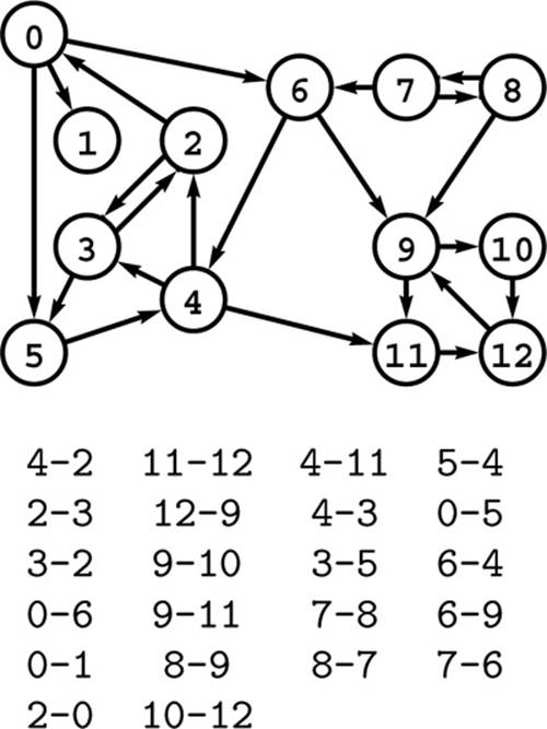
A digraph is defined by a list of nodes and edges (bottom), with the order that we list the nodes when specifying an edge implying that the edge is directed from the first node to the second. When drawing a digraph, we use arrows to depict directed edges (top).

We interpret edge directions in digraphs in many ways. For example, in a telephone-call graph, we might consider an edge to be directed from the caller to the person receiving the call. In a transaction graph, we might have a similar relationship where we interpret an edge as representing cash, goods, or information flowing from one entity to another. We find a modern situation that fits this classic model on the Internet, with vertices representing Web pages and edges the links between the pages. In Section 19.4, we examine other examples, many of which model situations that are more abstract.

One common situation is for the edge direction to reflect a precedence relationship. For example, a digraph might model a manufacturing line: Vertices correspond to jobs to be done, and an edge exists from vertex s to vertex t if the job corresponding to vertex s must be done before the job corresponding to vertex t. Another way to model the same situation is to use a PERT chart: edges represent jobs and vertices implicitly specify the precedence relationships (at each vertex, all incoming jobs must complete before any outgoing jobs can begin). How do we decide when to perform each of the jobs so that none of the precedence relationships are violated? This is known as a scheduling problem. It makes no sense if the digraph has a cycle so, in such situations, we are working with directed acyclic graphs (DAGs). We shall consider basic properties of DAGs and algorithms for this simple scheduling problem, which is known as topological sorting, in Sections 19.5 through 19.7. In practice, scheduling problems generally involve weights on the vertices or edges that model the time or cost of each job. We consider such problems in Chapters 21 and 22.

The number of possible digraphs is truly huge. Each of the V² possible directed edges (including self-loops) could be present or not, so the total number of different digraphs is 2^V2. As illustrated in Figure 19.2, this number grows very quickly, even by comparison with the number of different undirected graphs and even when V is small. As with undirected graphs, there is a much smaller number of classes of digraphs that are isomorphic to each other (the vertices of one can be relabeled to make it identical to the other), but we cannot take advantage of this reduction because we do not know an efficient algorithm for digraph isomorphism.

Figure 19.2 Graph enumeration

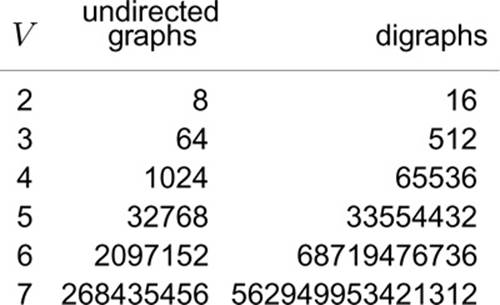
While the number of different undirected graphs with V vertices is huge, even when V is small, the number of different digraphs with V vertices is much larger. For undirected graphs, the number is given by the formula 2^V (V +1)/2; for digraphs, the formula is 2^V2.

Certainly, any program will have to process only a tiny fraction of the possible digraphs; indeed, the numbers are so large that we can be certain that virtually all digraphs will not be among those processed by any given program. Generally, it is difficult to characterize the digraphs that we might encounter in practice, so we design our algorithms such that they can handle any possible digraph as input. On the one hand, this situation is not new to us (for example, virtually none of the 1000! permutations of 1000 elements have ever been processed by any sorting program). On the other hand, it is perhaps unsettling to know that, for example, even if all the electrons in the universe could run supercomputers capable of processing 10¹⁰ graphs per second for the estimated lifetime of the universe, those supercomputers would see far fewer than 10⁻100 percent of the 10-vertex digraphs (see Exercise 19.9).

This brief digression on graph enumeration perhaps underscores several points that we cover whenever we consider the analysis of algorithms and indicates their particular relevance to the study of digraphs. Is it important to design our algorithms to perform well in the worst case, when we are so unlikely to see any particular worst-case digraph? Is it useful to choose algorithms on the basis of average-case analysis, or is that a mathematical fiction? If our intent is to have implementations that perform efficiently on digraphs that we see in practice, we are immediately faced with the problem of characterizing those digraphs. Mathematical models that can convincingly describe the digraphs that we might expect in applications are even more difficult to develop than are models for undirected graphs.

In this chapter, we revisit, in the context of digraphs, a subset of the basic graph-processing problems that we considered in Chapter 17, and we examine several problems that are specific to digraphs. In particular, we look at DFS and several of its applications, including cycle detection (to determine whether a digraph is a DAG);topological sort (to solve, for example, the scheduling problem for DAGs that was just described); and computation of the transitive closure and the strong components (which have to do with the basic problem of determining whether or not there is a directed path between two given vertices). As in other graph-processing domains, these algorithms range from the trivial to the ingenious; they are both informed by and give us insight into the complex combinatorial structure of digraphs.

Exercises

• 19.1 Find a large digraph somewhere online—perhaps a transaction graph in some online system, or a digraph defined by links on Web pages.

• 19.2 Find a large DAG somewhere online—perhaps one defined by function-definition dependencies in a large software system, or by directory links in a large file system.

19.3 Make a table like Figure 19.2, but exclude from the counts graphs and digraphs with self-loops.

19.4 How many digraphs are there that contain V vertices and E edges?

• 19.5 How many digraphs correspond to each undirected graph that contains V vertices and E edges?

• 19.6 How many digits do we need to express the number of digraphs that have V vertices as a base-10 number?

• 19.7 Draw the nonisomorphic digraphs that contain three vertices.

••• 19.8 How many different digraphs are there with V vertices and E edges if we consider two digraphs to be different only if they are not isomorphic?

• 19.9 Compute an upper bound on the percentage of 10-vertex digraphs that could ever be examined by any computer, under the assumptions described in the text and the additional ones that the universe has less than 10⁸⁰ electrons and that the age of the universe will be less than 10²⁰ years.