Algorithms Third Edition in C++ Part 5. Graph Algorithms (2006)
CHAPTER NINETEEN
Digraphs and DAGs
19.6 Topological Sorting
The goal of topological sorting is to be able to process the vertices of a DAG such that every vertex is processed before all the vertices to which it points. There are two natural ways to define this basic operation; they are essentially equivalent. Both tasks call for a permutation of the integers 0 through V-1, which we put in vertex-indexed vectors, as usual.
Topological sort (relabel) Given a DAG, relabel its vertices such that every directed edge points from a lower-numbered vertex to a higher-numbered one (see Figure 19.21).
Topological sort (rearrange) Given a DAG, rearrange its vertices on a horizontal line such that all the directed edges point from left to right (see Figure 19.22).
As indicated in Figure 19.22, it is easy to establish that the relabeling and rearrangement permutations are inverses of one another: Given a rearrangement, we can obtain a relabeling by assigning the label 0 to the first vertex on the list, 1 to the second label on the list, and so forth. For example, if a vector ts has the vertices in topologically sorted order, then the loop
Figure 19.22 Topological sorting (rearrangement)
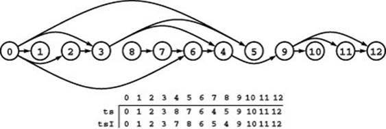
This diagram shows another way to look at the topological sort in Figure 19.21, where we specify a way to rearrange the vertices, rather than relabel them. When we place the vertices in the order specified in the array ts, from left to right, then all directed edges point from left to right. The inverse of the permutation ts is the permutation tsI that specifies the relabeling described in Figure 19.21.
for (i=0;i<V; i++) tsI[ts[i]] = i;
defines a relabeling in the vertex-indexed vector tsI. Conversely, we can get the rearrangement from the relabeling with the loop
for (i=0;i<V; i++) ts[tsI[i]] = i;
which puts the vertex that would have label 0 first in the list, the vertex that would have label 1 second in the list, and so forth. Most often, we use the term topological sort to refer to the rearrangement version of the problem. Note that ts is not a vertex-indexed vector.
In general, the vertex order produced by a topological sort is not unique. For example,
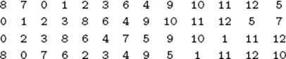
are all topological sorts of the example DAG in Figure 19.6 (and there are many others). In a scheduling application, this situation arises whenever one task has no direct or indirect dependence on another and thus they can be performed either before or after the other (or even in parallel). The number of possible schedules grows exponentially with the number of such pairs of tasks.
As we have noted, it is sometimes useful to interpret the edges in a digraph the other way around: We say that an edge directed from s to t means that vertex s “depends” on vertex t. For example, the vertices might represent terms to be defined in a book, with an edge from s to t if the definition of s uses t. In this case, it would be useful to find an ordering with the property that every term is defined before it is used in another definition. Using this ordering corresponds to positioning the vertices in a line such that edges all go from right to left—a reverse topological sort.Figure 19.23 illustrates a reverse topological sort of our sample DAG.
Figure 19.23 Reverse topological sort
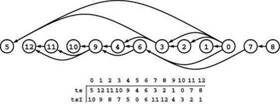
In this reverse topological sort of our sample digraph, the edges all point from right to left. Numbering the vertices as specified by the inverse permutation tsI gives a graph where every edge points from a higher-numbered vertex to a lower-numbered vertex.
Now, it turns out that we have already seen an algorithm for reverse topological sorting: our standard recursive DFS! When the input graph is a DAG, a postorder numbering puts the vertices in reverse topological order. That is, we number each vertex as the final action of the recursive DFS function, as in the post vector in the DFS implementation in Program 19.2. As illustrated in Figure 19.24, using this numbering is equivalent to numbering the nodes in the DFS forest in postorder, and gives a topological sort: The vertex-indexed vector post gives the relabeling and its inverse the rearrangement depicted in Figure 19.23—a reverse topological sort of the DAG.
Property 19.11 Postorder numbering in DFS yields a reverse topological sort for any DAG.
Proof: Suppose that s and t are two vertices such that s appears before t in the postorder numbering even though there is a directed edge s-t in the graph. Since we are finished with the recursive DFS for s at the time that we assign s its number, we have examined, in particular, the edge s-t. But if s-t were a tree, down, or cross edge, the recursive DFS for t would be complete, and t would have a lower number; however, s-t cannot be a back edge because that would imply a cycle. This contradiction implies that such an edge s-t cannot exist.
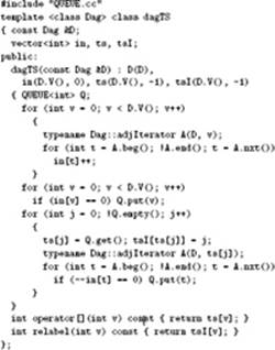
Thus, we can easily adapt a standard DFS to do a topological sort, as shown in Program 19.6. This implementation does a reverse topological sort: It computes the postorder numbering permutation and its inverse, so that clients can relabel or rearrange vertices.
Program 19.6 Reverse topological sort
This DFS class computes postorder numbering of the DFS forest (a reverse topological sort). Clients can use a TS object to relabel a DAG’s vertices so that every edge points from a higher-numbered vertex to a lower-numbered one or to arrange vertices such that the source vertex of every edge appears after the destination vertex (see Figure 19.23).
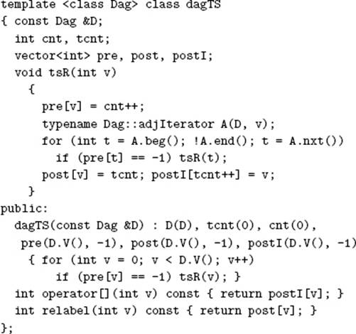
Figure 19.24 DFS forest for a DAG
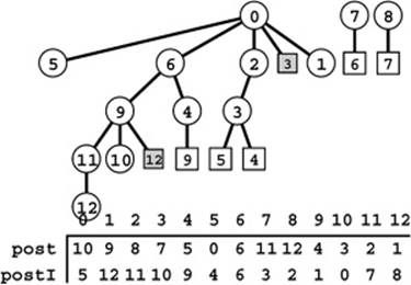
A DFS forest of a digraph has no back edges (edges to nodes with a higher postorder number) if and only if the digraph is a DAG. The non-tree edges in this DFS forest for the DAG of Figure 19.21 are either down edges (shaded squares) or cross edges (unshaded squares). The order in which vertices are encountered in a postorder walk of the forest, shown at the bottom, is a reverse topological sort (see Figure 19.23).
Computationally, the distinction between topological sort and reverse topological sort is not crucial. We can simply change the [] operator to return postI[G.V()-1 - v], or we can modify the implementation in one of the following ways:
• Do a reverse topological sort on the reverse of the given DAG.
• Rather than using it as an index for postorder numbering, push the vertex number on a stack as the final act of the recursive
Program 19.7 Topological sort
If we use this implementation of tsR in Program 19.6, the constructor computes a topological sort, not the reverse (for any DAG implementation that supports edge), because it replaces the reference to edge(v,w) in the DFS by edge(w, v), thus processing the reverse graph ( see text ).
void tsR(int v)
{
pre[v] = cnt++;
for (int w = 0; w < D.V(); w++)
if (D.edge(w, v))
if (pre[w] == -1) tsR(w);
post[v] = tcnt; postI[tcnt++] = v;
}
procedure. After the search is complete, pop the vertices from the stack. They come off the stack in topological order.
• Number the vertices in reverse order (start at V 1 and count down to 0). If desired, compute the inverse of the vertex numbering to get the topological order.
The proofs that these changes give a proper topological ordering are left for you to do as an exercise (see Exercise 19.97).
To implement the first of the options listed in the previous paragraph for sparse graphs (represented with adjacency lists), we would need to use Program 19.1 to compute the reverse graph. Doing so essentially doubles our space usage, which may thus become onerous for huge graphs. For dense graphs (represented with an adjacency matrix), as noted in Section 19.1, we can do DFS on the reverse without using any extra space or doing any extra work, simply by exchanging rows and columns when referring to the matrix, as illustrated in Program 19.7.
Next, we consider an alternative classical method for topological sorting that is more like breadth-first search (BFS) (see Section 18.7). It is based on the following property of DAGs.
Property 19.12 Every DAG has at least one source and at least one sink.
Figure 19.25 Topologically sorting a DAG by removing sources
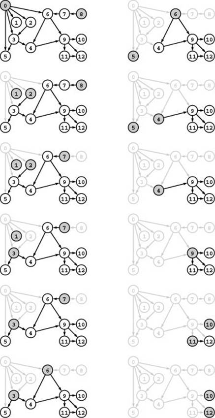
Since it is a source (no edges point to it), 0 can appear first in a topological sort of this example graph (left, top). If we remove 0 (and all the edges that point from it to other vertices), then 1 and 2 become sources in the resulting DAG (left, second from top), which we can then sort using the same algorithm. This figure illustrates the operation of Program 19.8, which picks from among the sources (the shaded nodes in each diagram) using the FIFO discipline, though any of the sources could be chosen at each step. See Figure 19.26 for the contents of the data structures that control the specific choices that the algorithm makes. The result of the topological sort illustrated here is the node order 082 1736 54 9111012.
Proof: Suppose that we have a DAG that has no sinks. Then, starting at any vertex, we can build an arbitrarily long directed path by following any edge from that vertex to any other vertex (there is at least one edge, since there are no sinks), then following another edge from that vertex, and so on. But once we have been to V +1 vertices, we must have seen a directed cycle, by the pigeonhole principle (see Property 19.6), which contradicts the assumption that we have a DAG. Therefore, every DAG has at least one sink. It follows that every DAG also has at least one source: its reverse’s sink.
From this fact, we can derive a topological-sort algorithm: Label any source with the smallest unused label, then remove it and label the rest of the DAG, using the same algorithm. Figure 19.25 is a trace of this algorithm in operation for our sample DAG.
Implementing this algorithm efficiently is a classic exercise in data-structure design ( see reference section ). First, there may be multiple sources, so we need to maintain a queue to keep track of them (any generalized queue will do). Second, we need to identify the sources in the DAG that remains when we remove a source. We can accomplish this task by maintaining a vertex-indexed vector that keeps track of the indegree of each vertex. Vertices with indegree 0 are sources, so we can initialize the queue with one scan through the DAG (using DFS or any other method that examines all of the edges). Then, we perform the following operations until the source queue is empty:
• Remove a source from the queue and label it.
• Decrement the entries in the indegree vector corresponding to the destination vertex of each of the removed vertex’s edges.
• If decrementing any entry causes it to become 0, insert the corresponding vertex onto the source queue.
Program 19.8 is an implementation of this method, using a FIFO queue, and Figure 19.26 illustrates its operation on our sample DAG, providing the details behind the dynamics of the example in Figure 19.25.
Figure 19.26 Indegree table and queue contents
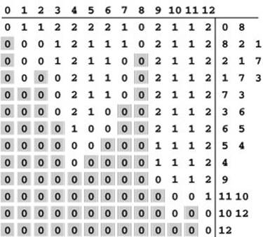
This sequence depicts the contents of the indegree table (left) and the source queue (right) during the execution of Program 19.8 on the sample DAG corresponding to Figure 19.25. At any given point in time, the source queue contains the nodes with indegree 0. Reading from top to bottom, we remove the leftmost node from the source queue, decrement the indegree entry corresponding to every edge leaving that node, and add any vertices whose entries become 0 to the source queue. For example, the second line of the table reflects the result of removing 0 from the source queue, then (because the DAG has the edges 0-1, 0-2, 0-3, 0-5, and 0-6) decrementing the indegree entries corresponding to 1, 2, 3, 5, and 6 and adding 2 and 1 to the source queue (because decrementing made their indegree entries 0). Reading the leftmost entries in the source queue from top to bottom gives a topological ordering for the graph.
The source queue does not empty until every vertex in the DAG is labeled, because the subgraph induced by the vertices not yet labeled is always a DAG, and every DAG has at least one source. Indeed, we can use the algorithm to test whether a graph is a DAG by inferring that there must be a cycle in the subgraph induced by the vertices not
Program 19.8 Source-queue–based topological sort
This class implements the same interface as does Programs 19.6 and 19.7. It maintains a queue of sources and uses a table that keeps track of the indegree of each vertex in the DAG induced by the vertices that have not been removed from the queue.
When we remove a source from the queue, we decrement the indegree entries corresponding to each of the vertices on its adjacency list (and put on the queue any vertices corresponding to entries that become 0). Vertices come off the queue in topologically sorted order.
yet labeled if the queue empties before all the vertices are labeled (see Exercise 19.104).
Processing vertices in topologically sorted order is a basic technique in processing DAGs. A classic example is the problem of finding the length of the longest path in a DAG. Considering the vertices in reverse topologically sorted order, the length of the longest path originating at each vertex v is easy to compute: Add one to the maximum of the lengths of the longest paths originating at each of the vertices reachable by a single edge from v. The topological sort ensures that all those lengths are known when v is processed, and that no other paths from v will be found afterwards. For example, taking a left-to-right scan of the reverse topological sort shown in Figure 19.23, we can quickly compute the following table of lengths of the longest paths originating at each vertex in the sample graph in Figure 19.21.
![]()
For example, the 6 corresponding to 0 (third column from the right) says that there is a path of length 6 originating at 0, which we know because there is an edge 0-2, we previously found the length of the longest path from 2 to be 5, and no other edge from 0 leads to a node having a longer path.
Whenever we use topological sorting for such an application, we have several choices in developing an implementation:
• Use DAGts in a DAG ADT, then proceed through the vector it computes to process the vertices.
• Process the vertices after the recursive calls in a DFS.
• Process the vertices as they come off the queue in a source-queue– based topological sort.
All of these methods are used in DAG-processing implementations in the literature, and it is important to know that they are all equivalent. We will consider other topological-sort applications in Exercises 19.111 and 19.114 and in Sections 19.7 and 21.4.
Exercises
• 19.92 Write a function that checks whether or not a given permutation of a DAG’s vertices is a proper topological sort of that DAG.
19.93 How many different topological sorts are there of the DAG that is depicted in Figure 19.6?
• 19.94 Give the DFS forest and the reverse topological sort that results from doing a standard adjacency-lists DFS (with postorder numbering) of the DAG
3-7 1-4 7-8 0-5 5-2 3-8 2-9 0-6 4-9 2-6 6-4 4-3 2-3.
• 19.95 Give the DFS forest and the topological sort that results from building a standard adjacency-lists representation of the DAG
3-7 1-4 7-8 0-5 5-2 3-8 2-9 0-6 4-9 2-6 6-4 4-3 2-3,
then using Program 19.1 to build the reverse, then doing a standard adjacency-lists DFS with postorder numbering.
• 19.96 Program 19.6 uses postorder numbering to do a reverse topological sort—why not use preorder numbering to do a topological sort? Give a three-vertex example that illustrates the reason.
• 19.97 Prove the correctness of each of the three suggestions given in the text for modifying DFS with postorder numbering such that it computes a topological sort instead of a reverse topological sort.
• 19.98 Give the DFS forest and the topological sort that results from doing a standard adjacency-matrix DFS with implicit reversal (and postorder numbering) of the DAG
3-7 1-4 7-8 0-5 5-2 3-8 2-9 0-6 4-9 2-6 6-4 4-3 2-3
(see Program 19.7).
• 19.99 Given a DAG, does there exist a topological sort that cannot result from applying a DFS-based algorithm, no matter what order the vertices adjacent to each vertex are chosen? Prove your answer.
• 19.100 Show, in the style of Figure 19.26, the process of topologically sorting the DAG
3-7 1-4 7-8 0-5 5-2 3-8 2-9 0-6 4-9 2-6 6-4 4-3 2-3
with the source-queue algorithm (Program 19.8).
• 19.101 Give the topological sort that results if the data structure used in the example depicted in Figure 19.25 is a stack rather than a queue.
• 19.102 Given a DAG, does there exist a topological sort that cannot result from applying the source-queue algorithm, no matter what queue discipline is used? Prove your answer.
19.103 Modify the source-queue topological-sort algorithm to use a generalized queue. Use your modified algorithm with a LIFO queue, a stack, and a randomized queue.
• 19.104 Use Program 19.8 to provide an implementation for a class for verifying that a DAG has no cycles (see Exercise 19.75).
• 19.105 Convert the source-queue topological-sort algorithm into a sink-queue algorithm for reverse topological sorting.
19.106 Write a program that generates all possible topological orderings of a given DAG, or, if the number of such orderings exceeds a bound taken as an argument, prints that number.
19.107 Write a program that converts any digraph with V vertices and E edges into a DAG by doing a DFS-based topological sort and changing the orientation of any back edge encountered. Prove that this strategy always produces a DAG.
•• 19.108 Write a program that produces each of the possible DAGs with V vertices and E edges with equal likelihood (see Exercise 17.70).
19.109 Give necessary and sufficient conditions for a DAG to have just one possible topologically sorted ordering of its vertices.
19.110 Run empirical tests to compare the topological-sort algorithms given in this section for various DAGs (see Exercise 19.2, Exercise 19.76, Exercise 19.107, and Exercise 19.108). Test your program as described in Exercise 19.11 (for low densities) and as described in Exercise 19.12 (for high densities).
• 19.111 Modify Program 19.8 so that it computes the number of different simple paths from any source to each vertex in a DAG.
• 19.112 Write a class that evaluates DAGs that represent arithmetic expressions (see Figure 19.19). Use a vertex-indexed vector to hold values corresponding to each vertex. Assume that values corresponding to leaves have been established.
• 19.113 Describe a family of arithmetic expressions with the property that the size of the expression tree is exponentially larger than the size of the corresponding DAG (so the running time of your program from Exercise 19.112 for the DAG is proportional to the logarithm of the running time for the tree).
• 19.114 Develop a method for finding the longest simple directed path in a DAG, in time proportional to V. Use your method to implement a class for printing a Hamilton path in a given DAG, if one exists.