Algorithms Third Edition in C++ Part 5. Graph Algorithms (2006)

CHAPTER TWENTY
Minimum Spanning Trees

20.3 Prim’s Algorithm and Priority-First Search

Prim’s algorithm is perhaps the simplest MST algorithm to implement, and it is the method of choice for dense graphs. We maintain a cut of the graph that is comprised of tree vertices (those chosen for the MST) and nontree vertices (those not yet chosen for the MST). We start by putting any vertex on the MST, then put a minimal crossing edge on the MST (which changes its nontree vertex to a tree vertex) and repeat the same operation V − 1 times, to put all vertices on the tree.

A brute-force implementation of Prim’s algorithm follows directly from this description. To find the edge to add next to the MST, we could examine all the edges that go from a tree vertex to a nontree vertex, then pick the shortest of the edges found to put on the MST. We do not consider this implementation here because it is overly expensive (see Exercises 20.35 through 20.37). Adding a simple data structure to eliminate excessive recomputation makes the algorithm both simpler and faster.

Adding a vertex to the MST is an incremental change: To implement Prim’s algorithm, we focus on the nature of that incremental change. The key is to note that our interest is in the shortest distance from each nontree vertex to the tree. When we add a vertex v to the tree, the only possible change for each nontree vertex w is that adding

Figure 20.8 Prim’s MST algorithm

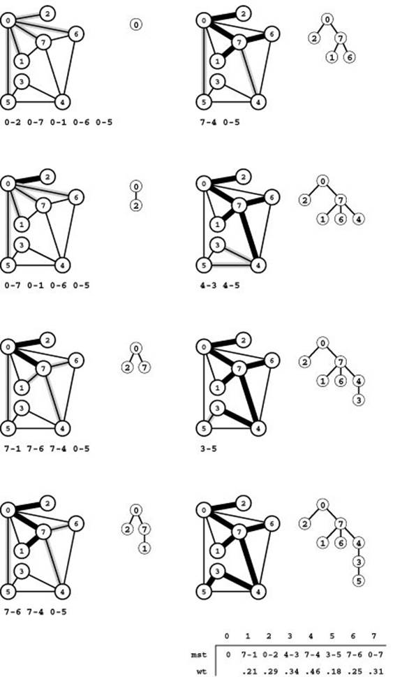
The first step in computing the MST with Prim’s algorithm is to add 0 to the tree. Then we find all the edges that connect 0 to other vertices (which are not yet on the tree) and keep track of the shortest (top left). The edges that connect tree vertices with nontree vertices (the fringe) are shadowed in gray and listed below each graph drawing. For simplicity in this figure, we list the fringe edges in order of their length so that the shortest is the first in the list. Different implementations of Prim’s algorithm use different data structures to maintain this list and to find the minimum. The second step is to move the shortest edge 0-2 (along with the vertex that it takes us to) from the fringe to the tree (second from top, left). Third, we move 0-7 from the fringe to the tree, replace 0-1 by 7-1 and 0-6 by 7-6 on the fringe (because adding 7 to the tree brings 1 and 6 closer to the tree), and add 7-4 to the fringe (because adding 7 to the tree makes 7-4 an edge that connects a tree vertex with a nontree vertex) (third from top, left). Next, we move edge 7-1 to the tree (bottom, left). To complete the computation, we take 7-6, 7-4, 4-3, and 3-5 off the queue, updating the fringe after each insertion to reflect any shorter or new paths discovered (right, top to bottom).
An oriented drawing of the growing MST is shown at the right of each graph drawing. The orientation is an artifact of the algorithm: We generally view the MST itself as a set of edges, unordered and unoriented.

v brings w closer than before to the tree. In short, we do not need to check the distance from w to all tree vertices—we just need to keep track of the minimum and check whether the addition of v to the tree necessitates that we update that minimum.

To implement this idea, we need data structures that can give us the following information:

• The tree edges

• The shortest edge connecting each nontree vertex to the tree

• The length of that edge

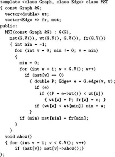
The simplest implementation for each of these data structures is a vertex-indexed vector (we can use such a vector for the tree edges by indexing on vertices as they are added to the tree). Program 20.6 is an implementation of Prim’s algorithm for dense graphs. It uses the vectors mst, fr, and wt (respectively) for these three data structures.

After adding a new edge (and vertex) to the tree, we have two tasks to accomplish:

• Check to see whether adding the new edge brought any nontree vertex closer to the tree.

• Find the next edge to add to the tree.

The implementation in Program 20.6 accomplishes both of these tasks with a single scan through the nontree vertices, updating wt[w] and fr[w] if v-w brings w closer to the tree, then updating the current minimum if wt[w] (the length of fr[w]) indicates that w is closer to the tree than any other nontree vertex with a lower index).

Property 20.6 Using Prim’s algorithm, we can find the MST of a dense graph in linear time.

Proof: It is immediately evident from inspection of the program that the running time is proportional to V² and therefore is linear for dense graphs.

Figure 20.8 shows an example MST construction with Prim’s algorithm; Figure 20.9 shows the evolving MST for a larger example.

Program 20.6 is based on the observation that we can interleave the find the minimum and update operations in a single loop where we examine all the nontree edges. In a dense graph, the number of edges that we may have to examine to update the distance from the nontree vertices to the tree is proportional to V, so looking at all the nontree edges to find the one that is closest to the tree does not represent

Figure 20.9 Prim’s MST algorithm

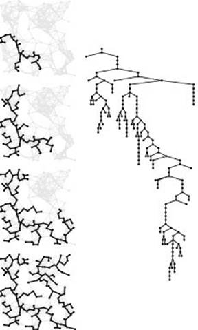
This sequence shows how the MST grows as Prim’s algorithm discovers 1/4, 1/2, 3/4, and all of the edges in the MST (top to bottom). An oriented representation of the full MST is shown at the right.

Program 20.6 Prim’s MST algorithm

This implementation of Prim’s algorithm is the method of choice for dense graphs and can be used for any graph representation that supports the edge existence test. The outer loop grows the MST by choosing a minimal edge crossing the cut between the vertices on the MST and vertices not on the MST. The w loop finds the minimal edge while at the same time (if w is not on the MST) maintaining the invariant that the edge fr[w] is the shortest edge (of weight wt[w]) from w to the MST.

The result of the computation is a vector of edge pointers. The first (mst[0]) is unused; the rest (mst[1] through mst[G.V()]) comprise the MST of the connected component of the graph that contains 0.

excessive extra cost. But in a sparse graph, we can expect to use substantially fewer than V steps to perform each of these operations. The crux of the strategy that we will use to do so is to focus on the set of potential edges to be added next to the MST—a set that we call the fringe. The number of fringe edges is typically substantially smaller than the number of nontree edges, and we can recast our description of the algorithm as follows. Starting with a self loop to a start vertex on the fringe and an empty tree, we perform the following operation until the fringe is empty:

Move a minimal edge from the fringe to the tree. Visit the vertex that it leads to, and put onto the fringe any edges that lead from that vertex to an nontree vertex, replacing the longer edge when two edges on the fringe point to the same vertex.

From this formulation, it is clear that Prim’s algorithm is nothing more than a generalized graph search (see Section 18.8), where the fringe is a priority queue based on a remove the minimum operation (see Chapter 9). We refer to generalized graph searching with priority queues as priority-first search (PFS). With edge weights for priorities, PFS implements Prim’s algorithm.

This formulation encompasses a key observation that we made already in connection with implementing BFS in Section 18.7. An even simpler general approach is to simply keep on the fringe all of the edges that are incident upon tree vertices, letting the priority-queue mechanism find the shortest one and ignore longer ones (see Exercise 20.41). As we saw with BFS, this approach is unattractive because the fringe data structure becomes unnecessarily cluttered with edges that will never get to the MST. The size of the fringe could grow to be proportional to E (with whatever attendant costs having a fringe this size might involve), while the PFS approach just outlined ensures that the fringe will never have more than V entries.

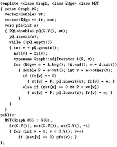
As with any implementation of a general algorithm, we have a number of available approaches for interfacing with priority-queue ADTs. One approach is to use a priority queue of edges, as in our generalized graph-search implementation of Program 18.10. Program 20.7 is an implementation that is essentially equivalent to Program 18.10 but uses a vertex-based approach so that it can use an indexed priority-queue, as described in Section 9.6. (We consider a complete implemen tation of the specific priority-queue interface used by Program 20.7 is at the end of this chapter, inProgram 20.10.) We identify the fringe vertices, the subset of nontree vertices that are connected by fringe edges to tree vertices, and keep the same vertex-indexed vectors mst, fr, and wt as in Program 20.6. The priority queue contains the index of each fringe vertex, and that entry gives access to the shortest edge connecting the fringe vertex with the tree and the length of that edge, through the second and third vectors.

The first call to pfs in the constructor in Program 20.7 finds the MST in the connected component that contains vertex 0, and subsequent calls find MSTs in other components, so this class actually finds minimal spanning forests in graphs that are not connected (see Exercise 20.34).

Property 20.7 Using a PFS implementation of Prim’s algorithm that uses a heap for the priority-queue implementation, we can compute an MST in time proportional to E lg V.

Proof: The algorithm directly implements the generic idea of Prim’s algorithm (add next to the MST a minimal edge that connects a vertex on the MST with a vertex not on the MST). Each priority-queue operation requires less than lg V steps. Each vertex is chosen with a remove the minimum operation; and, in the worst case, each edge might require a change priority operation.

Priority-first search is a proper generalization of breadth-first and depth-first search because those methods also can be derived through appropriate priority settings. For example, we can (somewhat artificially) use a variable cnt to assign a unique priority cnt++ to each vertex when we put that vertex on the priority queue. If we define P to be cnt, we get preorder numbering and DFS because newly encountered nodes have the highest priority. If we define P to be V-cnt, we get BFS because old nodes have the highest priority. These priority assignments make the priority queue operate like a stack and a queue, respectively. This equivalence is purely of academic interest since the priority-queue operations are unnecessary for DFS and BFS. Also, as discussed in Section 18.8, a formal proof of equivalence would require a precise attention to replacement rules to obtain the same sequence of vertices as result from the classical algorithms.

Program 20.7 Priority-first search

The function pfs is a generalized graph search that uses a priority queue for the fringe (see Section 18.8). The priority P is defined such that this class implements Prim’s MST algorithm; other priority definitions give other algorithms. The main loop moves the highest-priority (lowest-weight) edge from the fringe to the tree, then checks every edge adjacent to the new tree vertex to see whether it implies changes in the fringe. Edges to vertices not on the fringe or the tree are added to the fringe; shorter edges to fringe vertices replace corresponding fringe edges.

The PQi class is an indirect priority-queue interface (see Section 9.6) modified to pass a reference to the priority array to the constructor, to substitute getmin for delmax, and to substitute lower for change. Program 20.10 is an implementation of this interface.

As we shall see, PFS encompasses not just DFS, BFS, and Prim’s MST algorithm but also several other classical algorithms. The various algorithms differ only in their priority functions. Thus, the running times of all these algorithms depend on the performance of the priority-queue ADT. Indeed, we are led to a general result that encompasses not just the two implementations of Prim’s algorithms that we have examined in this section but also a broad class of fundamental graph-processing algorithms.

Property 20.8 For all graphs and all priority functions, we can compute a spanning tree with PFS in linear time plus time proportional to the time required for V insert, V delete the minimum, and E decrease key operations in a priority queue of size at most V.

Proof: The proof of Property 20.7 establishes this more general result. We have to examine all the edges in the graph; hence the “linear time” clause. The algorithm never increases the priority (it changes the priority to only a lower value); by more precisely specifying what we need from the priority-queue ADT ( decrease key, not necessarily change priority ), we strengthen this statement about performance.

In particular, use of an unordered-array priority-queue implementation gives an optimal solution for dense graphs that has the same worst-case performance as the classical implementation of Prim’s algorithm (Program 20.6). That is, Properties 20.6 and 20.7 are special cases of Property 20.8; throughout this book we shall see numerous other algorithms that essentially differ in only their choice of priority function and their priority-queue implementation.

Property 20.7 is an important general result: The time bound stated is a worst-case upper bound that guarantees performance within a factor of lg V of optimal (linear time) for a large class of graph-processing problems. Still, it is somewhat pessimistic for many of the graphs that we encounter in practice, for two reasons. First, the lg V bound for priority-queue operation holds only when the number of vertices on the fringe is proportional to V, and even then it is just an upper bound. For a real graph in a practical application, the fringe might be small (see Figures 20.10 and 20.11), and some priority-queue operations might take many fewer than lg V steps. Although noticeable, this effect is likely to account for only a small constant factor in the running time; for example, a proof that the fringe never has more than pV vertices on it would improve the bound by only a factor of 2. More important, we generally perform many fewer than E decrease key operations since we do that operation only when we find an edge to a fringe node that is shorter than the current best-known edge to a fringe node. This event is relatively rare: Most edges have no effect on the priority queue (see Exercise 20.40). It is reasonable to regard PFS as an essentially linear-time algorithm unless V lg V is significantly greater than E.

Figure 20.10 PFS implementation of Prim’s MST algorithm

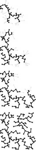
With PFS, Prim’s algorithm processes just the vertices and edges closest to the MST (in gray).

Figure 20.11 Fringe size for PFS implementation of Prim’s algorithm

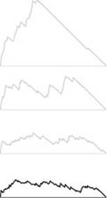
The plot at the bottom shows the size of the fringe as the PFS proceeds for the example in Figure 20.10. For comparison, the corresponding plots for DFS, randomized search, and BFS from Figure 18.28 are shown above in gray.

The priority-queue ADT and generalized graph-searching abstractions make it easy for us to understand the relationships among various algorithms. Since these abstractions (and software mechanisms to support their use) were developed many years after the basic methods, relating the algorithms to classical descriptions of them becomes an exercise for historians. However, knowing basic facts about the history is useful when we encounter descriptions of MST algorithms in the research literature or in other texts, and understanding how these few simple abstractions tie together the work of numerous researchers over a time span of decades is persuasive evidence of their value and power. Thus, we consider briefly the origins of these algorithms here.

An MST implementation for dense graphs essentially equivalent to Program 20.6 was first presented by Prim in 1961, and, independently, by Dijkstra soon thereafter. It is usually referred to as Prim’s algorithm, although Dijkstra’s presentation was more general, so some scholars refer to the MST algorithm as a special case of Dijkstra’s algorithm. But the basic idea was also presented by Jarnik in 1939, so some authors refer to the method as Jarnik’s algorithm, thus characterizing Prim’s (or Dijkstra’s) role as finding an efficient implementation of the algorithm for dense graphs. As the priority-queue ADT came into use in the early 1970s, its application to finding MSTs of sparse graphs was straightforward; the fact that MSTs of sparse graphs could be computed in time proportional to E lg V became widely known without attribution to any particular researcher. Since that time, as we discuss in Section 20.6, many researchers have concentrated on finding efficient priority-queue implementations as the key to finding efficient MST algorithms for sparse graphs.

Exercises

• 20.35 Analyze the performance of the brute-force implementation of Prim’s algorithm mentioned at the beginning of this section for a complete weighted graph with V vertices. Hint: The following combinatorial sum might be useful:Σ^1k<V k (V−k) = (V+1) V (V−1) /6.

• 20.36 Answer Exercise 20.35 for graphs in which all vertices have the same fixed degree t.

• 20.37 Answer Exercise 20.35 for general sparse graphs that have V vertices and E edges. Since the running time depends on the weights of the edges and on the degrees of the vertices, do a worst-case analysis. Exhibit a family of graphs for which your worst-case bound is confirmed.

20.38 Show, in the style of Figure 20.8, the result of computing the MST of the network defined in Exercise 20.26 with Prim’s algorithm.

• 20.39 Describe a family of graphs with V vertices and E edges for which the worst-case running time of the PFS implementation of Prim’s algorithm is confirmed.

•• 20.40 Develop a reasonable generator for random graphs with V vertices and E edges such that the running time of the PFS implementation of Prim’s algorithm (Program 20.7) is nonlinear.

• 20.41 Modify Program 20.7 so that it works like Program 18.8, in that it keeps on the fringe all edges incident upon tree vertices. Run empirical studies to compare your implementation with Program 20.7, for various weighted graphs (see Exercises 20.9–14).

20.42 Derive a priority queue implementation for use by Program 20.7 from the interface defined in Program 9.12 (so any implementation of that interface could be used).

20.43 Use the STL priority_queue to implement the priority-queue interface that is used by Program 20.7.

20.44 Suppose that you use a priority-queue implementation that maintains a sorted list. What would be the worst-case running time for graphs with V vertices and E edges, to within a constant factor? When would this method be appropriate, if ever? Defend your answer.

• 20.45 An MST edge whose deletion from the graph would cause the MST weight to increase is called a critical edge. Show how to find all critical edges in a graph in time proportional to E lg V.

20.46 Run empirical studies to compare the performance of Program 20.6 to that of Program 20.7, using an unordered array implementation for the priority queue, for various weighted graphs (see Exercises 20.9–14).

• 20.47 Run empirical studies to determine the effect of using an index-heap– tournament (see Exercise 9.53) priority-queue implementation instead of Program 9.12 in Program 20.7, for various weighted graphs (see Exercises 20.9– 14).

20.48 Run empirical studies to analyze tree weights (see Exercise 20.23) as a function of V, for various weighted graphs (see Exercises 20.9–14).

20.49 Run empirical studies to analyze maximum fringe size as a function of V, for various weighted graphs (see Exercises 20.9–14).

20.50 Run empirical studies to analyze tree height as a function of V, for various weighted graphs (see Exercises 20.9–14).

20.51 Run empirical studies to study the dependence of the results of Exercises 20.49 and 20.50 on the start vertex. Would it be worthwhile to use a random starting point?

• 20.52 Write a client program that does dynamic graphical animations of Prim’s algorithm. Your program should produce images like Figure 20.10 (see Exercises 17.56 through 17.60). Test your program on random Euclidean neighbor graphs and on grid graphs (see Exercises 20.17 and20.19), using as many points as you can process in a reasonable amount of time.