Algorithms Third Edition in C++ Part 5. Graph Algorithms (2006)
CHAPTER TWENTY
Minimum Spanning Trees
20.4 Kruskal’s Algorithm
Prim’s algorithm builds the MST one edge at a time, finding a new edge to attach to a single growing tree at each step. Kruskal’s algorithm also builds the MST one edge at a time; but, by contrast, it finds an edge that connects two trees in a spreading forest of growing MST subtrees. We start with a degenerate forest of V single-vertex trees and perform the operation of combining two trees (using the shortest edge possible) until there is just one tree left: the MST.
Figure 20.12 shows a step-by-step example of the operation of Kruskal’s algorithm; Figure 20.13 illustrates the algorithm’s dynamic characteristics on a larger example. The disconnected forest of MST subtrees evolves gradually into a tree. Edges are added to the MST in order of their length, so the forests comprise vertices that are connected to one another by relatively short edges. At any point during the execution of the algorithm, each vertex is closer to some vertex in its subtree than to any vertex not in its subtree.
Kruskal’s algorithm is simple to implement, given the basic algorithmic tools that we have considered in this book. Indeed, we can use any sort from Part 3 to sort the edges by weight and any of the connectivity algorithms from Chapter 1 to eliminate those that cause cycles! Program 20.8 is an implementation along these lines of an MST function for a graph ADT that is functionally equivalent to the other MST implementations that we consider in this chapter. The implementation does not depend on the graph representation: It calls a GRAPH client to return a vector that contains the graph’s edges, then computes the MST from that vector.
Figure 20.12 Kruskal’s MST algorithm
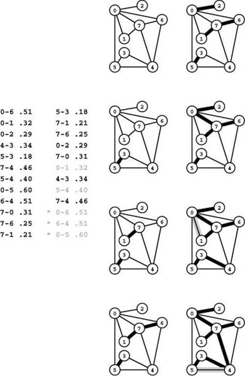
Given a list of a graph’s edges in arbitrary order (left edge list), the first step in Kruskal’s algorithm is to sort them by weight (right edge list). Then we go through the edges on the list in order of their weight, adding edges that do not create cycles to the MST. We add 5-3 (the shortest edge), then 7-1, then 7-6 (left), then 0-2 (right, top) and 0-7 (right, second from top). The edge with the next largest weight, 0-1, creates a cycle and is not included. Edges that we do not add to the MST are shown in gray on the sorted list. Then we add 4-3 (right, third from top). Next, we reject 5-4 because it causes a cycle, then we add 7-4 (right, bottom). Once the MST is complete, any edges with larger weights would cause cycles and be rejected (we stop when we have added V-1 edges to the MST). These edges are marked with asterisks on the sorted list.
Note that there are two ways in which Kruskal’s algorithm can terminate. If we find V − 1 edges, then we have a spanning tree and can stop. If we examine all the edges without finding V −1 tree edges, then we have determined that the graph is not connected, precisely as we did in Chapter 1.
Analyzing the running time of Kruskal’s algorithm is a simple matter because we know the running time of its constituent ADT operations.
Property 20.9 Kruskal’s algorithm computes the MST of a graph in time proportional to E lg E.
Proof: This property is a consequence of the more general observation that the running time of Program 20.8 is proportional to the cost of sorting E numbers plus the cost of E find and V − 1 union operations. If we use standard ADT implementations such as mergesort and weighted union-find with halving, the cost of sorting dominates.
We consider the comparative performance of Kruskal’s and Prim’s algorithm in Section 20.6. For the moment, note that a running time proportional to E lg E is not necessarily worse than E lg V, because E is at most V2, so lg E is at most 2lg V. Performance differences for specific graphs are due to what the properties of the implementations are and to whether the actual running time approaches these worst-case bounds.
In practice, we might use quicksort or a fast system sort (which is likely to be based on quicksort). Although this approach may give the usual unappealing (in theory) quadratic worst case for the sort, it is likely to lead to the fastest run time. Indeed, on the other hand, we could use a radix sort to do the sort in linear time (under certain conditions on the weights) so that the cost of the E find operations dominates and then adjust Property 20.9 to say that the running time of Kruskal’s algorithm is within a constant factor of E lg*E under those conditions on the weights (see Chapter 2). Recall that the function lg*E is the number of iterations of the binary logarithm function before the result is less than 1, which is less than 5 if E is less than 265536. In other words, these adjustments make Kruskal’s algorithm effectively linear in most practical circumstances.
Figure 20.13 Kruskal’s MST algorithm
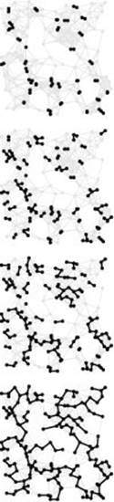
This sequence shows 1 / 4, 1 / 2, 3 / 4, and the full MST as it evolves.
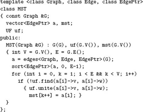
Program 20.8 Kruskal’s MST algorithm
This implementation uses our sorting ADT from Chapter 6 and our union-find ADT from Chapter 4 to find the MST by considering the edges in order of their weights, discarding edges that create cycles until finding V − 1 edges that comprise a spanning tree.
Not shown are a wrapper class EdgePtr that wraps pointers to Edges so sort can compare them using an overloaded <, as described in Section 6.8, and a version of Program 20.2 with a third template argument.
Typically, the cost of finding the MST with Kruskal’s algorithm is even lower than the cost of processing all edges because the MST is complete well before a substantial fraction of the (long) graph edges is ever considered. We can take this fact into account to reduce the running time significantly in many practical situations by keeping edges that are longer than the longest MST edge entirely out of the sort. One easy way to accomplish this objective is to use a priority queue, with an implementation that does the construct operation in linear time and the remove the minimum operation in logarithmic time.
For example, we can achieve these performance characteristics with a standard heap implementation, using bottom-up construction (see Section 9.4). Specifically, we make the following changes to Program 20.8: First, we change the call on sort to a call on pq.construct() to build a heap in time proportional to E. Second, we change the inner loop to take the shortest edge off the priority queue with e = pq.delmin() and to change all references to a[i] to refer to e.
Property 20.10 A priority-queue–based version of Kruskal’s algorithm computes the MST of a graph in time proportional to E + X lg V, where X is the number of graph edges not longer than the longest edge in the MST.
Proof: See the preceding discussion, which shows the cost to be the cost of building a priority queue of size E plus the cost of running the X delete the minimum, X find, and V −1 union operations. Note that the priority-queue–construction costs − dominate (and the algorithm is linear time) unless X is greater than E/ lg V.
We can also apply the same idea to reap similar benefits in a quicksort-based implementation. Consider what happens when we use a straight recursive quicksort, where we partition at i, then recursively sort the subfile to the left of i and the subfile to the right of i. We note that, by construction of the algorithm, the first i elements are in sorted order after completion of the first recursive call (see Program 9.2). This obvious fact leads immediately to a fast implementation of Kruskal’s algorithm: If we put the check for whether the edge a[i] causes a cycle between the recursive calls, then we have an algorithm that, by construction, has checked the first i edges, in sorted order, after completion of the first recursive call! If we include a test to return when we have found V-1 MST edges, then we have an algorithm that sorts only as many edges as we need to compute the MST, with a few extra partitioning stages involving larger elements (see Exercise 20.57). Like straight sorting implementations, this algorithm could run in quadratic time in the worst case, but we can provide a probabilistic guarantee that the worst-case running time will not come close to this limit. Also, like straight sorting implementations, this program is likely to be faster than a heap-based implementation because of its shorter inner loop.
If the graph is not connected, the partial-sort versions of Kruskal’s algorithm offer no advantage because all the edges have to be considered. Even for a connected graph, the longest edge in the graph might be in the MST, so any implementation of Kruskal’s method would still have to examine all the edges. For example, the graph might consist of tight clusters of vertices all connected together by short edges, with one outlier connected to one of the vertices by a long edge. Despite such anomalies, the partial-sort approach is probably worthwhile because it offers significant gain when it applies and incurs little if any extra cost.
Historical perspective is relevant and instructive here as well. Kruskal presented this algorithm in 1956, but, again, the relevant ADT implementations were not carefully studied for many years, so the performance characteristics of implementations such as the priority-queue version ofProgram 20.8 were not well understood until the 1970s. Other interesting historical notes are that Kruskal’s paper mentioned a version of Prim’s algorithm (see Exercise 20.59) and that Boruvka mentioned both approaches. Efficient implementations of Kruskal’s method for sparse graphs preceded implementations of Prim’s method for sparse graphs because union-find (and sort) ADTs came into use before priority-queue ADTs. Generally, as was true of implementations of Prim’s algorithm, advances in the state of the art for Kruskal’s algorithm are attributed primarily to advances in ADT performance. On the other hand, the applicability of the union-find abstraction to Kruskal’s algorithm and the applicability of the priority-queue abstraction to Prim’s algorithm have been prime motivations for many researchers to seek better implementations of those ADTs.
Exercises
• 20.53 Show, in the style of Figure 20.12, the result of computing the MST of the network defined in Exercise 20.26 with Kruskal’s algorithm.
• 20.54 Run empirical studies to analyze the length of the longest edge in the MST and the number of graph edges that are not longer than that one, for various weighted graphs (see Exercises 20.9–14).
• 20.55 Develop an implementation of the union-find ADT that implements find in constant time and union in time proportional to lg V.
20.56 Run empirical tests to compare your ADT implementation from Exercise 20.55 to weighted union-find with halving (Program 1.4) when Kruskal’s algorithm is the client, for various weighted graphs (see Exercises 20.9–14). Separate out the cost of sorting the edges so that you can study the effects of the change both on the total cost and on the part of the cost associated with the union-find ADT.
20.57 Develop an implementation based on the idea described in the text where we integrate Kruskal’s algorithm with quicksort so as to check MST membership of each edge as soon as we know that all smaller edges have been checked.
• 20.58 Adapt Kruskal’s algorithm to implement two ADT functions that fill a client-supplied vertex-indexed vector classifying vertices into k clusters with the property that no edge of length greater than d connects two vertices in different clusters. For the first function, take k as an argument and return d; for the second, take d as an argument and return k. Test your program on random Euclidean neighbor graphs and on grid graphs (see Exercises 20.17 and 20.19) of various sizes for various values of k and d.
20.59 Develop an implementation of Prim’s algorithm that is based on pre-sorting the edges.
• 20.60 Write a client program that does dynamic graphical animations of Kruskal’s algorithm (see Exercise 20.52). Test your program on random Euclidean neighbor graphs and on grid graphs (see Exercises 20.17 and 20.19), using as many points as you can process in a reasonable amount of time.
Figure 20.14 Boruvka’s MST algorithm
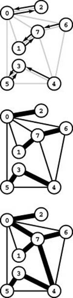
The diagram at the top shows a directed edge from each vertex to its closest neighbor. These edges show that 0-2, 1-7, and 3-5 are each the shortest edge incident on both their vertices, 6-7 is 6’s shortest edge, and 4-3 is 4’s shortest edge. These edges all belong to the MST and comprise a forest of MST subtrees (center), as computed by the first phase of Boruvka’s algorithm. In the second phase, the algorithm completes the MST computation (bottom) by adding the edge 0-7, which is the shortest edge incident on any of the vertices in the subtrees it connects, and the edge 4-7, which is the shortest edge incident on any of the vertices in the bottom subtree.
All materials on the site are licensed Creative Commons Attribution-Sharealike 3.0 Unported CC BY-SA 3.0 & GNU Free Documentation License (GFDL)
If you are the copyright holder of any material contained on our site and intend to remove it, please contact our site administrator for approval.
© 2016-2025 All site design rights belong to S.Y.A.