Algorithms Third Edition in C++ Part 5. Graph Algorithms (2006)

CHAPTER TWENTY
Minimum Spanning Trees

20.5 Boruvka’s Algorithm

The next MST algorithm that we consider is also the oldest. Like Kruskal’s algorithm, we build the MST by adding edges to a spreading forest of MST subtrees; but we do so in stages, adding several MST edges at each stage. At each stage, we find the shortest edge that connects each MST subtree with a different one, then add all such edges to the MST.

Again, our union-find ADT from Chapter 1 leads to an efficient implementation. For this problem, it is convenient to extend the interface to make the find operation available to clients. We use this function to associate an index with each subtree so that we can tell quickly to which subtree a given vertex belongs. With this capability, we can implement efficiently each of the necessary operations for Boruvka’s algorithm.

First, we maintain a vertex-indexed vector that identifies, for each MST subtree, the nearest neighbor. Then, we perform the following operations on each edge in the graph:

• If it connects two vertices in the same tree, discard it.

• Otherwise, check the nearest-neighbor distances between the two trees the edge connects and update them if appropriate.

After this scan of all the graph edges, the nearest-neighbor vector has the information that we need to connect the subtrees. For each vertex index, we perform a union operation to connect it with its nearest neighbor. In the next stage, we discard all the longer edges that connect other pairs of vertices in the now-connected MST subtrees. Figures 20.14 and 20.15 illustrate this process on our sample algorithm

Program 20.9 is a direct implementation of Boruvka’s algorithm. There are three major factors that make this implementation efficient:

• The cost of each find operation is essentially constant.

• Each stage decreases the number of MST subtrees in the forest by at least a factor of 2.

• A substantial number of edges is discarded during each stage. It is difficult to quantify precisely all these factors, but the following bound is easy to establish.

Property 20.11 The running time of Boruvka’s algorithm for computing the MST of a graph is O ( E lg V lg^*E) .

Proof: Since the number of trees in the forest is halved at each stage, the number of stages is no larger than lg V. The time for each stage is at most proportional to the cost of E find operations, which is less than E lg^*E, or linear for practical purposes.

The running time given in Property 20.11 is a conservative upper bound since it does not take into account the substantial reduction in the number of edges during each stage. The find operations take constant time in the early passes, and there are very few edges in the later passes. Indeed, for many graphs, the number of edges decreases exponentially with the number of vertices, and the total running time is proportional to E. For example, as illustrated in Figure 20.16, the algorithm finds the MST of our larger sample graph in just four stages.

It is possible to remove the lg^*E factor to lower the theoretical bound on the running time of Boruvka’s algorithm to be proportional to E lg V, by representing MST subtrees with doubly-linked lists instead of using the union and find operations. However, this improvement is sufficiently more complicated to implement and the potential performance improvement sufficiently marginal that it is not likely to be worth considering for use in practice (see Exercises 20.66 and 20.67).

Figure 20.15 Union-find array in Boruvka’s algorithm

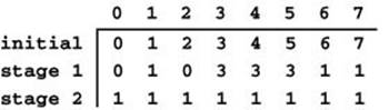
This figure depicts the contents of the union-find array corresponding to the example depicted in Figure 20.14. Initially, each entry contains its own index, indicating a forest of singleton vertices. After the first stage, we have three components, represented by the indices 0, 1, and 3 (the union-find trees are all flat for this tiny example). After the second stage, we have just one component, represented by 1.

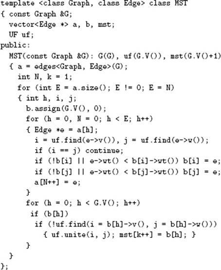
Program 20.9 Boruvka’s MST algorithm

This implementation of Boruvka’s MST algorithm uses a version of the union-find ADT from Chapter 4 (with a single-argument find added to the interface) to associate indices with MST subtrees as they are built. Each phase checks all the remaining edges; those that connect disjoint subtrees are kept for the next phase. The array a has the edges not yet discarded and not yet in the MST. The index N is used to store those being saved for the next phase (the code resets E from N at the end of each phase) and the index h is used to access the next edge to be checked. Each component’s nearest neighbor is kept in the array b with find component numbers as indices. At the end of each phase, each component is united with its nearest neighbor and the nearest-neighbor edges added to the MST.

As we mentioned, Boruvka’s is the oldest of the algorithms that we consider: It was originally conceived in 1926, for a power-distribution application. The method was rediscovered by Sollin in 1961; it later attracted attention as the basis for MST algorithms with efficient asymptotic performance and as the basis for parallel MST algorithms.

Exercises

• 20.61 Show, in the style of Figure 20.14, the result of computing the MST of the network defined in Exercise 20.26 with Boruvka’s algorithm.

• 20.62 Why does Program 20.9 do a find test before doing the union operation? Hint: Consider equal-length edges.

• 20.63 Explain why b(h) could be null in the test in Program 20.9 that guards the union operation.

• 20.64 Describe a family of graphs with V vertices and E edges for which the number of edges that survive each stage of Boruvka’s algorithm is sufficiently large that the worst-case running time is achieved.

20.65 Develop an implementation of Boruvka’s algorithm that is based on a presorting of the edges.

• 20.66 Develop an implementation of Boruvka’s algorithm that uses doubly-linked circular lists to represent MST subtrees, so that subtrees can be merged and renamed in time proportional to E during each stage (and the equivalence-relations ADT is therefore not needed).

• 20.67 Do empirical studies to compare your implementation of Boruvka’s algorithm in Exercise 20.66 with the implementation in the text (Program 20.9), for various weighted graphs (see Exercises 20.9–14).

• 20.68 Do empirical studies to tabulate the number of stages and the number of edges processed per stage in Boruvka’s algorithm, for various weighted graphs (see Exercises 20.9–14).

20.69 Develop an implementation of Boruvka’s algorithm that constructs a new graph (one vertex for each tree in the forest) at each stage.

• 20.70 Write a client program that does dynamic graphical animations of Boruvka’s algorithm (see Exercises 20.52 and 20.60). Test your program on random Euclidean neighbor graphs and on grid graphs (see Exercises 20.17 and 20.19), using as many points as you can process in a reasonable amount of time.

Figure 20.16 Boruvka’s MST algorithm

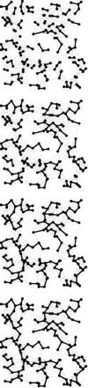
The MST evolves in just four stages for this example (top to bottom).