Algorithms Third Edition in C++ Part 5. Graph Algorithms (2006)
CHAPTER TWENTY-ONE
Shortest Paths
21.3 All-Pairs Shortest Paths
In this section, we consider two classes that solve the all-pairs shortest-paths problem. The algorithms that we implement directly generalize two basic algorithms that we considered in Section 19.3 for the transitive-closure problem. The first method is to run Dijkstra’s algorithm from each vertex to get the shortest paths from that vertex to each of the others. If we implement the priority queue with a heap, the worst-case running time for this approach is proportional to V E lg V, and we can improve this bound to V E for many types of networks by using a d-ary heap. The second method, which allows us to solve the problem directly in time proportional to V3, is an extension of Warshall’s algorithm that is known as Floyd’s algorithm.
Both of these classes implement an abstract–shortest-paths ADT interface for finding shortest distances and paths. This interface, which is shown in Program 21.2, is a generalization to weighted digraphs of the abstract–transitive-closure interface for connectivity queries in digraphs that we studied in Chapter 19. In both class implementations, the constructor solves the all-pairs shortest-paths problem and saves the result in private data members to support query functions that return the shortest-path length from one given vertex to another and either the first or last edge on the path. Implementing such an ADT is a primary reason to use all-pairs shortest-paths algorithms in practice.
Program 21.3 is a sample client program that uses the all– shortest-paths ADT interface to find the weighted diameter of a network. It checks all pairs of vertices to find the one for which the shortest-path length is longest; then, it traverses the path, edge by edge. Figure 21.13 shows the path computed by this program for our Euclidean network example.
Figure 21.13 Diameter of a network
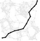
The largest entry in a network’s all-shortest-paths matrix is the diameter of the network: the length of the longest of the shortest paths, depicted here for our sample Euclidean network.
The goal of the algorithms in this section is to support constant-time implementations of the query functions. Typically, we expect to have a huge number of such requests, so we are willing to invest substantial resources in private data members and preprocessing in the constructor to be able to answer the queries quickly. Both of the algorithms that we consider use space proportional to V2 for the private data members.
The primary disadvantage of this general approach is that, for a huge network, we may not have so much space available (or we might
Program 21.2 All-pairs shortest-paths ADT
Our solutions to the all-pairs shortest-paths problem are all classes with a constructor and two query functions: a dist function that returns the length of the shortest path from the first argument to the second; and one of two possible path functions, either path, which returns a pointer to the first edge on the shortest path, or pathR, which returns a pointer to the final edge on the shortest path. If there is no such path, the path function returns 0 and dist is undefined.
We use path or pathR as convenient for the algorithm under scrutiny; in practice, we might need to settle upon one or the other (or both) in the interface and use various transfer functions in implementations, as discussed in Section 21.1 and in the exercises at the end of this section.
template <class Graph, class Edge> class SPall
{
public:
SPall(const Graph &);
Edge *path(int, int) const;
Edge *pathR(int, int) const;
double dist(int, int) const;
};
not be able to afford the requisite preprocessing time). In principle, our interface provides us with the latitude to trade off preprocessing time and space for query time. If we expect only a few queries, we can do no preprocessing and simply run a single-source algorithm for each query, but intermediate situations require more advanced algorithms (see Exercises 21.48 through 21.50). This problem generalizes one that challenged us for much of Chapter 19: the problem of supporting fast reachability queries in limited space.
The first all-pairs shortest-paths ADT function implementation that we consider solves the problem by using Dijkstra’s algorithm to solve the single-source problem for each vertex. In C++, we can express the method directly, as shown in Program 21.4: We build a vector of SPT objects, one to solve the single-source problem for each vertex. This method generalizes the BFS-based method for unweighted undirected graphs that we considered in Section 17.7. It is also similar
Program 21.3 Computing the diameter of a network
This client function illustrates the use of the interface in Program 21.2. It finds the longest of the shortest paths in the given network, prints the path, and returns its weight (the diameter of the network).
template <class Graph, class Edge>
double diameter(Graph &G)
{ int vmax = 0, wmax = 0;
allSP<Graph, Edge> all(G);
for (int v = 0; v < G.V(); v++)
for (int w = 0; w < G.V(); w++)
if (all.path(v, w))
if (all.dist(v, w) > all.dist(vmax, wmax))
{ vmax = v; wmax = w; }
int v = vmax; cout << v;
while (v != wmax)
{ v = all.path(v, wmax)->w(); cout << ”-” << v; }
return all.dist(vmax, wmax);
}
to our use of a DFS that starts at each vertex to compute the transitive closure of unweighted digraphs, in Program 19.4.
Property 21.7 With Dijkstra’s algorithm, we can find all shortest paths in a network that has nonnegative weights in time proportional to V E logd V, where d = 2if E < 2V, and d =E/V otherwise.
Proof: Immediate from Property 21.6.
As are our bounds for the single-source shortest-paths and the MST problems, this bound is conservative; and a running time of V E is likely for typical graphs.
To compare this implementation with others, it is useful to study the matrices implicit in the vector-of-vectors structure of the private data members. The wt vectors form precisely the distances matrix that we considered in Section 21.1: The entry in row s and column t is the length of the shortest path from s to t. As illustrated in Figures 21.8 and 21.9, the spt vectors from the transpose of the paths matrix: The entry in row s and column t is the last entry on the shortest path from s to t.
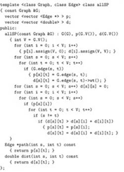
Program 21.4 Dijkstra’s algorithm for all shortest paths
This class uses Dijkstra’s algorithm to build an SPT for each vertex so that it can answer pathR and dist queries for any pair of vertices.
#include “SPT.cc”
template <class Graph, class Edge> class allSP
{ const Graph &G;
vector< SPT<Graph, Edge> *> A;
public:
allSP(const Graph &G) : G(G), A(G.V())
{ for (int s = 0; s < G.V(); s++)
A[s] = new SPT<Graph, Edge>(G, s); }
Edge *pathR(int s, int t) const
{ return A[s]->pathR(t); }
double dist(int s, int t) const
{ return A[s]->dist(t); }
};
For dense graphs, we could use an adjacency-matrix representation and avoid computing the reverse graph by implicitly transposing the matrix (interchanging the row and column indices), as in Program 19.7. Developing an implementation along these lines is an interesting programming exercise and leads to a compact implementation (see Exercise 21.43); however, a different approach, which we consider next, admits an even more compact implementation.
The method of choice for solving the all-pairs shortest-paths problem in dense graphs, which was developed by R. Floyd, is precisely the same as Warshall’s method, except that instead of using the logical or operation to keep track of the existence of paths, it checks distances for each edge to determine whether that edge is part of a new shorter path. Indeed, as we have noted, Floyd’s and Warshall’s algorithms are identical in the proper abstract setting (see Sections 19.3 and 21.1).
Program 21.5 is an all-pairs shortest-paths ADT function that implements Floyd’s algorithm. It explictly uses the matrices from Section 21.1 as private data members: a V -by-V vector of vectors d for the distances matrix, and another V -by-V vector of vectors p for the paths table. For every pair of vertices s and t, the constructor sets
Program 21.5 Floyd’s algorithm for all shortest paths
This implementation of the interface in Program 21.2 uses Floyd’s algorithm, a generalization of Warshall’s algorithm (see Program 19.3) that finds the shortest paths between each pair of points instead of just testing for their existence.
After initializing the distances and paths matrices with the graph’s edges, we do a series of relaxation operations to compute the shortest paths. The algorithm is simple to implement, but verifying that it computes the shortest paths is more complicated (see text).
d[s][t] to the shortest-path length from s to t (to be returned by the dist member function) and p[s][t] to the index of the next vertex on the shortest path from s to t (to be returned by the path member function). The implementation is based upon the path relaxation operation that we considered in Section 21.1.
Property 21.8With Floyd’s algorithm, we can find all shortest paths in a network in time proportional to V3.
Proof: The running time is immediate from inspection of the code. We prove that the algorithm is correct by induction in precisely the same way as we did for Warshall’s algorithm. The ith iteration of the loop computes a shortest path from s to t in the network that does not include any vertices with indices greater than i (except possibly the endpoints s and t). Assuming this fact to be true for the ith iteration of the loop, we prove it to be true for the (i+1)st iteration of the loop. A shortest path from s to t that does not include any vertices with indices greater than i+1 is either (i) a path from s to t that does not include any vertices with indices greater than i, of length d[s][t], that was found on a previous iteration of the loop, by the inductive hypothesis; or (ii) comprising a path from s to i and a path from i to t, neither of which includes any vertices with indices greater than i, in which case the inner loop sets d[s][t].
Figure 21.14 is a detailed trace of Floyd’s algorithm on our sample network. If we convert each blank entry to 0 (to indicate the absence of an edge) and convert each nonblank entry to 1 (to indicate the presence of an edge), then these matrices describe the operation of Warshall’s algorithm in precisely the same manner as we did in Figure 19.15. For Floyd’s algorithm, the nonblank entries indicate more than the existence of a path; they give information about the shortest known path. An entry in the distance matrix has the length of the shortest known path connecting the vertices corresponding to the given row and column; the corresponding entry in the paths matrix gives the next vertex on that path. As the matrices become filled with nonblank entries, running Warshall’s algorithm amounts to just double-checking that new paths connect pairs of vertices already known to be connected by a path; in contrast, Floyd’s algorithm must compare (and update if necessary) each new path to see whether the new path leads to shorter paths.
Figure 21.14 Floyd’s algorithm
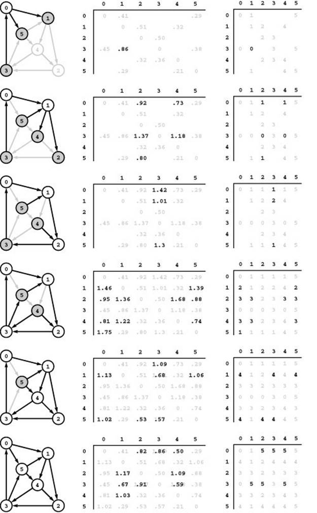
This sequence shows the construction of the all-pairs shortest-paths matrices with Floyd’s algorithm. For i from 0 to 5 (top to bottom), we consider, for all s and t, all of the paths from s to t having no intermediate vertices greater than i (the shaded vertices). Initially, the only such paths are the network’s edges, so the distances matrix (center) is the graph’s adjacency matrix and the paths matrix (right) is set with p[s][t] = t for each edge s-t. For vertex 0 (top), the algorithm finds that 3-0-1 is shorter than the sentinel value that is present because there is no edge 3-1 and updates the matrices accordingly. It does not do so for paths such as 3-0-5, which is not shorter than the known path 3-5. Next the algorithm considers paths through 0 and 1 (second from top) and finds the new shorter paths 0-1-2, 0-1-4, 3-0-1-2, 3-0-1-4, and 5-1-2. The third row from the top shows the updates corresponding to shorter paths through 0, 1, and 2 and so forth.
Black numbers overstriking gray ones in the matrices indicate situations where the algorithm finds a shorter path than one it found earlier. For example, .91 overstrikes 1.37 in row 3 and column 2 in the bottom diagram because the algorithm discovered that 3-5-4-2 is shorter than 3-0-1-2.
Comparing the worst-case bounds on the running times of Dijkstra’s and Floyd’s algorithms, we can draw the same conclusion for these all-pairs shortest-paths algorithms as we did for the corresponding transitive-closure algorithms in Section 19.3. Running Dijkstra’s algorithm on each vertex is clearly the method of choice for sparse networks, because the running time is close to V E. As density increases, Floyd’s algorithm—which always takes time proportional to V3—becomes competitive (see Exercise 21.67); it is widely used because it is so simple to implement.
A more fundamental distinction between the algorithms, which we examine in detail in Section 21.7, is that Floyd’s algorithm is effective in even those networks that have negative weights (provided that there are no negative cycles). As we noted in Section 21.2, Dijkstra’s method does not necessarily find shortest paths in such graphs.
The classical solutions to the all-pairs shortest-paths problem that we have described presume that we have space available to hold the distances and paths matrices. Huge sparse graphs, where we cannot afford to have any V-by-V matrices, present another set of challenging and interesting problems. As we saw in Chapter 19, it is an open problem to reduce this space cost to be proportional to V while still supporting constant-time shortest-path-length queries. We found the analogous problem to be difficult even for the simpler reachability problem (where we are satisfied with learning in constant time whether there is any path connecting a given pair of vertices), so we cannot expect a simple solution for the all-pairs shortest-paths problem. Indeed, the number of different shortest path lengths is, in general, proportional to V2 even for sparse graphs. That value, in some sense, measures the amount of information that we need to process, and perhaps indicates that when we do have restrictions on space, we must expect to spend more time on each query (see Exercises 21.48 through 21.50).
Exercises
• 21.39 Estimate, to within a factor of 10, the largest graph (measured by its number of vertices) that your computer and programming system could handle if you were to use Floyd’s algorithm to compute all its shortest paths in 10 seconds.
• 21.40 Estimate, to within a factor of 10, the largest graph of density 10 (measured by its number of edges) that your computer and programming system could handle if you were to use Dijkstra’s algorithm to compute all its shortest paths in 10 seconds.
21.41 Show, in the style of Figure 21.9, the result of using Dijkstra’s algorithm to compute all shortest paths of the network defined in Exercise 21.1.
21.42 Show, in the style of Figure 21.14, the result of using Floyd’s algorithm to compute all shortest paths of the network defined in Exercise 21.1.
• 21.43 Combine Program 20.6 and Program 21.4 to make an implementation of the all-pairs shortest-paths ADT interface (based on Dijkstra’s algorithm) for dense networks that supports path queries but does not explicitly compute the reverse network. Do not define a separate function for the single-source solution—put the code from Program 20.6 directly in the inner loop and put results directly in private data members d and p like those in Program 21.5).
21.44 Run empirical tests, in the style of Table 20.2, to compare Dijkstra’s algorithm (Program 21.4 and Exercise 21.43) and Floyd’s algorithm (Pro-gram 21.5), for various networks (see Exercises 21.4–8).
21.45 Run empirical tests to determine the number of times that Floyd’s and Dijkstra’s algorithms update the values in the distances matrix, for various networks (see Exercises 21.4–8).
21.46 Give a matrix in which the entry in row s and column t is equal to the number of different simple directed paths connecting s and t in Figure 21.1.
21.47 Implement a class whose constructor computes the path-count matrix that is described in Exercise 21.46 so that it can provide count queries through a public member function in constant time.
• 21.48 Develop a class implementation of the abstract–shortest-paths ADT for sparse graphs that cuts the space cost to be proportional to V, by increasing the query time to be proportional to V.
• 21.49 Develop a class implementation of the abstract–shortest-paths ADT for sparse graphs that uses substantially less than O (V2) space but supports queries in substantially less than O (V ) time. Hint: Compute all shortest paths for a subset of the vertices.
• 21.50 Develop a class implementation of the abstract–shortest-paths ADT for sparse graphs that uses substantially less than O (V2) space and (using randomization) supports queries in constant expected time.
• 21.51 Develop a class implementation of the abstract–shortest-paths ADT that takes the lazy approach of using Dijkstra’s algorithm to build the SPT (and associated distance vector) for each vertex s the first time that the client issues a shortest-path query from s, then references the information on subsequent queries.
21.52 Modify the shortest-paths ADT and Dijkstra’s algorithm to handle shortest-paths computations in networks that have weights on both vertices and edges. Do not rebuild the graph representation (the method described in Exercise 21.4); modify the code instead.
• 21.53 Build a small model of airline routes and connection times, perhaps based upon some flights that you have taken. Use your solution to Exercise 21.52 to compute the fastest way to get from one of the served destinations to another. Then test your program on real data (see Exercise 21.5).