Algorithms Third Edition in C++ Part 5. Graph Algorithms (2006)
CHAPTER TWENTY-ONE
Shortest Paths
21.4 Shortest Paths in Acyclic Networks
In Chapter 19, we found that, despite our intuition that DAGs should be easier to process than general digraphs, developing algorithms with substantially better performance for DAGs than for general digraphs is an elusive goal. For shortest-paths problems, we do have algorithms for DAGs that are simpler and faster than the priority-queue–based methods that we have considered for general digraphs. Specifically, in this section we consider algorithms for acyclic networks that
• Solve the single-source problem in linear time.
• Solve the all-pairs problem in time proportional to V E.
• Solve other problems, such as finding longest paths.
In the first two cases, we cut the logarithmic factor from the running time that is present in our best algorithms for sparse networks; in the third case, we have simple algorithms for problems that are intractable for general networks. These algorithms are all straightforward extensions to the algorithms for reachability and transitive closure in DAGs that we considered in Chapter 19.
Since there are no cycles at all, there are no negative cycles; so negative weights present no difficulty in shortest-paths problems on DAGs. Accordingly, we place no restrictions on edge-weight values throughout this section.
Next, a note about terminology: We might choose to refer to directed graphs with weights on the edges and no cycles either as weighted DAGs or as acyclic networks. We use both terms interchangeably to emphasize their equivalence and to avoid confusion when we refer to the literature, where both are widely used. It is sometimes convenient to use the former to emphasize differences from unweighted DAGs that are implied by weights and the latter to emphasize differences from general networks that are implied by acyclicity.
The four basic ideas that we applied to derive efficient algorithms for unweighted DAGs in Chapter 19 are even more effective for weighted DAGs.
• Use DFS to solve the single-source problem.
• Use a source queue to solve the single-source problem.
• Invoke either method, once for each vertex, to solve the all-pairs problem.
• Use a single DFS (with dynamic programming) to solve the all-pairs problem.
These methods solve the single-source problem in time proportional to E and the all-pairs problem in time proportional to V E. They are all effective because of topological ordering, which allows us compute shortest paths for each vertex without having to revisit any decisions. We consider one implementation for each problem in this section; we leave the others for exercises (see Exercises 21.62 through 21.65).
We begin with a slight twist. Every DAG has at least one source but could have several, so it is natural to consider the following shortest-paths problem.
Multisource shortest paths Given a set of start vertices, find, for each other vertex w, a shortest path among the shortest paths from each start vertex to w.
This problem is essentially equivalent to the single-source shortest-paths problem. We can convert a multisource problem into a single-source problem by adding a dummy source vertex with zero-length edges to each source in the network. Conversely, we can convert a single-source problem to a multisource problem by working with the induced subnetwork defined by all the vertices and edges reachable from the source. We rarely construct such subnetworks explicitly, because our algorithms automatically process them if we treat the start vertex as though it were the only source in the network (even when it is not).
Topological sorting immediately presents a solution to the multi-source shortest-paths problem and to numerous other problems. We maintain a vertex-indexed vector wt that gives the weight of the shortest known path from any source to each vertex. To solve the multisource shortest-paths problem, we initialize the wt vector to 0 for sources and a large sentinel value for all the other vertices. Then, we process the vertices in topological order. To process a vertex v, we perform a relaxation operation for each outgoing edge v-w that updates the shortest path to w if v-w gives a shorter path from a source to w (through v). This process checks all paths from any source to each vertex in the graph; the relaxation operation keeps track of the minimum-length such path, and the topological sort ensures that we process the vertices in an appropriate order.
We can implement this method directly in one of two ways. The first is to add a few lines of code to the topological sort code in Program 19.8: Just after we remove a vertex v from the source queue, we perform the indicated relaxation operation for each of its edges (see Exercise 21.56). The second is to put the vertices in topological order, then to scan through them and to perform the relaxation operations precisely as described in the previous paragraph.
These same processes (with other relaxation operations) can solve many graph-processing problems. For example, Program 21.6 is an implementation of the second approach (sort, then scan) for solving the multisource longest-paths problem: For each vertex in the network, what is a longest path from some source to that vertex? We interpret the wt entry associated with each vertex to be the length of the longest known path from any source to that vertex, initialize all of the weights to 0, and change the sense of the comparison in the relaxation operation. Figure 21.15 traces the operation of Program 21.6 on a sample acyclic network.
Property 21.9We can solve the multisource shortest-paths problem and the multisource longest-paths problem in acyclic networks in linear time.
Proof: The same proof holds for longest path, shortest path, and many other path properties. To match Program 21.6, we state the proof for longest paths. We show by induction on the loop variable i that, for all vertices v = ts[j] with j < i that have been processed, wt[v] is the length of the longest path from a source to v. When v = ts[i], let t be the vertex preceding v on any path from a source to v. Since vertices in the ts vector are in topologically sorted order, t must have been processed already. By the induction hypothesis, wt[t] is the length of the longest path to t, and the relaxation step in the code checks whether that path gives a longer path to v through t. The induction hypothesis also implies that all paths to v are checked in this way as v is processed.
This property is significant because it tells us that processing acyclic networks is considerably easier than processing networks that
Figure 21.15 Computing longest paths in an acyclic network
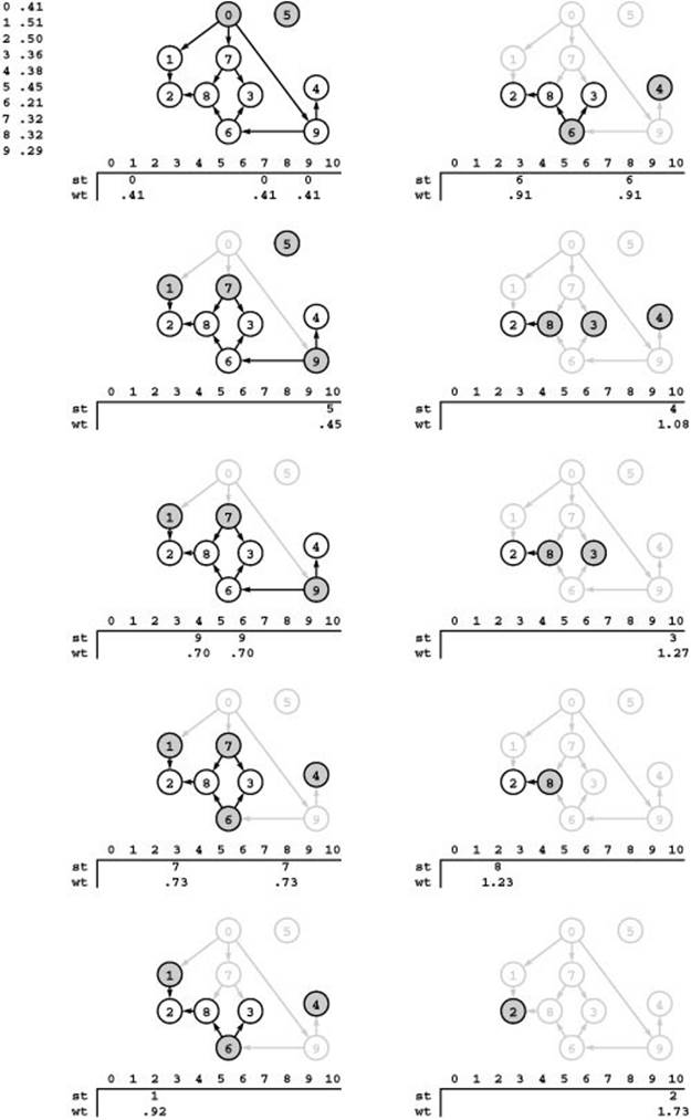
In this network, each edge has the weight associated with the vertex that it leads from, listed at the top left. Sinks have edges to a dummy vertex 10, which is not shown in the drawings. The wt array contains the length of the longest known path to each vertex from some source, and the st array contains the previous vertex on the longest path. This figure illustrates the operation of Program 21.6, which picks from among the sources (the shaded nodes in each diagram) using the FIFO discipline, though any of the sources could be chosen at each step. We begin by removing 0 and checking each of its incident edges, discovering one-edge paths of length .41 to 1, 7, and 9. Next, we remove 5 and record the one-edge path from 5 to 10 (left, second from top). Next, we remove 9 and record the paths 0-9-4 and 0-9-6, of length .70 (left, third from top). We continue in this way, changing the arrays whenever we find longer paths. For example, when we remove 7 (left, second from bottom) we record paths of length .73 to 8 and 3; then, later, when we remove 6, we record longer paths (of length .91) to 8 and 3 (right, top). The point of the computation is to find the longest path to the dummy node 10. In this case, the result is the path 0-9-6-8-2, of length 1.73.
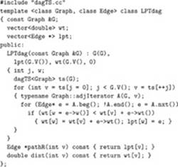
Program 21.6 Longest paths in an acyclic network
To find the longest paths in an acyclic network, we consider the vertices in topological order, keeping the weight of the longest known path to each vertex in a vertex-indexed vector wt by doing a relaxation step for each edge. The vector lpt defines a a spanning forest of longest paths (rooted at the sources) so that path(v) returns the last edge on the longest path to v.
have cycles. For shortest paths, the method is faster than Dijkstra’s algorithm by a factor proportional to the cost of the priority-queue operations in Dijkstra’s algorithm. For longest paths, we have a linear algorithm for acyclic networks but an intractable problem for general networks. Moreover, negative weights present no special difficulty here, but they present formidable barriers for algorithms on general networks, as discussed in Section 21.7.
The method just described depends on only the fact that we process the vertices in topological order. Therefore, any topological-sorting
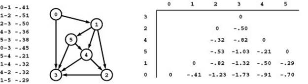
Figure 21.16 Shortest paths in an acyclic network
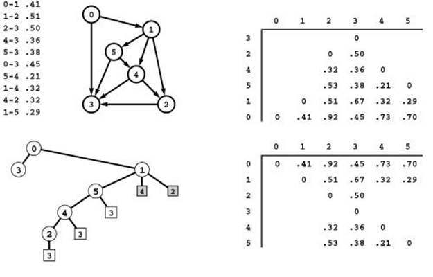
This diagram depicts the computation of the all-shortest-distances matrix (bottom right) for a sample weighted DAG (top left), computing each row as the last action in a recursive DFS function. Each row is computed from the rows for adjacent vertices, which appear earlier in the list, because the rows are computed in reverse topological order (postorder traversal of the DFS tree shown at the bottom left). The array on the top right shows the rows of the matrix in the order that they are computed. For example, to compute each entry in the row for 0 we add .41 to the corresponding entry in the row for 1 (to get the distance to it from 0 after taking 0-1), then add .45 to the corresponding entry in the row for 3 (to get the distance to it from 0 after taking 0-3), and take the smaller of the two. The computation is essentially the same as computing the transitive closure of a DAG (see, for example, Figure 19.23). The most significant difference between the two is that the transitive-closure algorithm could ignore down edges (such as 1-2 in this example) because they go to vertices known to be reachable, while the shortest-paths algorithm has to check whether paths associated with down edges are shorter than known paths. If we were to ignore 1-2 in this example, we would miss the shortest paths 0-1-2 and 1-2.
algorithm can be adapted to solve shortest- and longest-paths problems and other problems of this type (see, for example, Exercises 21.56 and 21.62).
As we know from Chapter 19, the DAG abstraction is a general one that arises in many applications. For example, we see an application in Section 21.6 that seems unrelated to networks but that can be addressed directly with Program 21.6.
Next, we turn to the all-pairs shortest-paths problem for acyclic networks. As in Section 19.3, one method that we could use to solve this problem is to run a single-source algorithm for each vertex (see Exercise 21.65). The equally effective approach that we consider here is to use a single DFS with dynamic programming, just as we did for computing the transitive closure of DAGs in Section 19.5 (see Program 19.9). If we consider the vertices at the end of the recursive function, we are processing them in reverse topological order and can derive the shortest-path vector for each vertex from the shortest-path vectors for each adjacent vertex, simply by using each edge in a relaxation step.
Program 21.7 is an implementation along these lines. The operation of this program on a sample weighted DAG is illustrated in Figure 21.16. Beyond the generalization to include relaxation, there is one important difference between this computation and the transitiveclosure
Program 21.7 All shortest paths in an acyclic network
This implementation of the interface in Program 21.2 for weighted DAGs is derived by adding appropriate relaxation operations to the dynamic-programming–based transitive-closure function in Program 19.9.
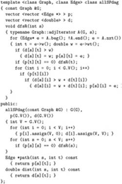
Figure 21.17 All longest paths in an acyclic network
Our method for computing all shortest paths in acyclic networks works even if the weights are negative. Therefore, we can use it to compute longest paths, simply by first negating all the weights, as illustrated here for the network in Figure 21.16. The longest simple path in this network is 0-1-5-4-2-3, of weight 1.73.
computation for DAGs: In Program 19.9, we had the choice of ignoring down edges in the DFS tree because they provide no new information about reachability; in Program 21.7, however, we need to consider all edges, because any edge might lead to a shorter path.
Property 21.10 We can solve the all-pairs shortest-paths problem in acyclic networks with a single DFS in time proportional to V E.
Proof: This fact follows immediately from the strategy of solving the single-source problem for each vertex (see Exercise 21.65). We can also establish it by induction, from Program 21.7. After the recursive calls for a vertex v, we know that we have computed all shortest paths for each vertex on v’s adjacency list, so we can find shortest paths from v to each vertex by checking each of v’s edges. We do V relaxation steps for each edge, for a total of V E relaxation steps.
Thus, for acyclic networks, topological sorting allows us to avoid the cost of the priority queue in Dijkstra’s algorithm. Like Floyd’s algorithm, Program 21.7 also solves problems more general than those solved by Dijkstra’s algorithm, because, unlike Dijkstra’s (see Section 21.7), this algorithm works correctly even in the presence of negative edge weights. If we run the algorithm after negating all the weights in an acyclic network, it finds all longest paths, as depicted in Figure 21.17. Or, we can find longest paths by reversing the inequality test in the relaxation algorithm, as in Program 21.6.
The other algorithms for finding shortest paths in acyclic networks that are mentioned at the beginning of this section generalize the methods from Chapter 19 in a manner similar to the other algorithms that we have examined in this chapter. Developing implementations of them is a worthwhile way to cement your understanding of both DAGs and shortest paths (see Exercises 21.62 through 21.65). All the methods run in time proportional to V E in the worst case, with actual costs dependent on the structure of the DAG. In principle, we might do even better for certain sparse weighted DAGs (see Exercise 19.117).
Exercises
• 21.54 Give the solutions to the multisource shortest- and longest-paths problems for the network defined in Exercise 21.1, with the directions of edges 2-3 and 1-0 reversed.
• 21.55 Modify Program 21.6 such that it solves the multisource shortest-paths problem for acyclic networks.
• 21.56 Implement a class with the same interface as Program 21.6 that is derived from the source-queue–based topological-sorting code of Program 19.8, performing the relaxation operations for each vertex just after that vertex is removed from the source queue.
• 21.57 Define an ADT for the relaxation operation, provide implementations, and modify Program 21.6 to use your ADT such that you can use Program 21.6 to solve the multisource shortest-paths problem, the multisource longest-paths problem, and other problems, just by changing the relaxation implementation.
21.58 Use your generic implementation from Exercise 21.57 to implement a class with member functions that return the length of the longest paths from any source to any other vertex in a DAG, the length of the shortest such path, and the number of vertices reachable via paths whose lengths fall within a given range.
• 21.59 Define properties of relaxation such that you can modify the proof of Property 21.9 to apply an abstract version of Program 21.6 (such as the one described in Exercise 21.57).
• 21.60 Show, in the style of Figure 21.16, the computation of the all-pairs shortest-paths matrices for the network defined in Exercise 21.54 by Program 21.7.
• 21.61 Give an upper bound on the number of edge weights accessed by Program 21.7, as a function of basic structural properties of the network. Write a program to compute this function, and use it to estimate the accuracy of the V E bound, for various acyclic networks (add weights as appropriate to the models in Chapter 19).
• 21.62 Write a DFS-based solution to the multisource shortest-paths problem for acyclic networks. Does your solution work correctly in the presence of negative edge weights? Explain your answer.
• 21.63 Extend your solution to Exercise 21.62 to provide an implementation of the all-pairs shortest-paths ADT interface for acyclic networks that builds the all-paths and all-distances matrices in time proportional to V E.
21.64 Show, in the style of Figure 21.9, the computation of all shortest paths of the network defined in Exercise 21.54 using the DFS-based method of Exercise 21.63.
• 21.65 Modify Program 21.6 such that it solves the single-source shortest-paths problem in acyclic networks, then use it to develop an implementation of the all-pairs shortest-paths ADT interface for acyclic networks that builds the all-paths and all-distances matrices in time proportional toV E.
• 21.66 Work Exercise 21.61 for the DFS-based (Exercise 21.63) and for the topological-sort–based (Exercise 21.65) implementations of the all-pairs shortest-paths ADT. What inferences can you draw about the comparative costs of the three methods?
21.67 Run empirical tests, in the style of Table 20.2, to compare the three class implementations for the all-pairs shortest-paths problem described in this section (see Program 21.7, Exercise 21.63, and Exercise 21.65), for various acyclic networks (add weights as appropriate to the models inChapter 19)