Algorithms Third Edition in C++ Part 5. Graph Algorithms (2006)
CHAPTER TWENTY-TWO
Network Flow
22.5 Mincost Flows
It is not unusual for there to be numerous solutions to a given maxflow problem. This fact leads to the question of whether we might wish to impose some additional criteria for choosing one of them. For example, there are clearly many solutions to the unit-capacity flow problems shown in Program 22.22; perhaps we would prefer the one that uses the fewest edges or the one with the shortest paths, or perhaps we would like to know whether there exists one comprising disjoint paths. Such problems are more difficult than the standard maxflow problem; they fall into a more general model known as the mincost flow problem, which is the subject of this section.
As with the maxflow problem, there are numerous equivalent ways to pose the mincost-flow problem. We consider one standard formulation in detail in this section, then consider various reductions in Section 22.7.
Specifically, we use the mincost-maxflow model: We define an edge type that includes integer costs, use the edge costs to define a flow cost in a natural way, then ask for a maximal flow of minimal cost. As we learn, not only do we have efficient and effective algorithms for this problem, but also the problem-solving model is of broad applicability.
Definition 22.8 The flow cost of an edge in a flow network with edge costs is the product of that edge’s flow and cost. The cost of a flow is the sum of the flow costs of that flow’s edges.
We continue to assume that capacities are positive integers less than M. We also assume edge costs to be nonnegative integers less than C. (Disallowing negative costs is primarily a matter of convenience, as discussed in Section 22.7.) As before, we assign names to these upper-bound values because the running times of some algorithms depend on the latter. With these basic assumptions, the problem that we wish to solve is trivial to define.
Mincost maxflow Given a flow network with edge costs, find a maxflow such that no other maxflow has lower cost.
Figure 22.40 illustrates different maxflows in a flow network with costs, including a mincost maxflow. Certainly, the computational burden of minimizing cost is no less challenging than the burden of maximizing flow with which we were concerned in Sections 22.2
Figure 22.40 Maxflows in flow networks with costs
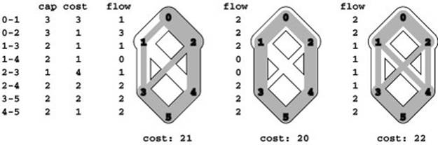
These flows all have the same (maximal) value, but their costs (the sum of the products of edge flows and edge costs) differ. The maxflow in the center has minimal cost (no maxflow has lower cost).
and 22.3. Indeed, costs add an extra dimension that presents significant new challenges. Even so, we can shoulder this burden with a generic algorithm that is similar to the augmenting-path algorithm for the maxflow problem.
Numerous other problems reduce to or are equivalent to the mincost-maxflow problem. For example, the following formulation is of interest because it encompasses the merchandise-distribution problem that we considered at the beginning of the chapter.
Mincost feasible flow Recall that we define a flow in a network with vertex weights (supply if positive, demand if negative) to be feasible if the sum of the vertex weights is negative and the difference between each vertex’s outflow and inflow. Given such a network, find a feasible flow of minimal cost.
To describe the network model for the mincost–feasible-flow problem, we use the term distribution network for brevity to mean “capacitated flow network with edge costs and supply or demand weights on vertices.”
In the merchandise-distribution application, supply vertices correspond to warehouses, demand vertices to retail outlets, edges to trucking routes, supply or demand values to the amount of material to be shipped or received, and edge capacities to the number and capacity of the trucks available for the various routes. A natural way to interpret each edge’s cost is as the cost of moving a unit of flow through that edge (the cost of sending a unit of material in a truck along the corresponding route). Given a flow, an edge’s flow cost is the part of the cost of moving the flow through the network that we can attribute to that edge. Given an amount of material that is to be shipped along a given edge, we can compute the cost of shipping it by multiplying the cost per unit by the amount. Doing this computation for each edge
Program 22.8 Computing flow cost
This function, which might be added to Program 22.1, returns the cost of a network’s flow. It sums cost times flow for all positive-capacity edges, allowing for uncapacitated edges to be used as dummy edges.
static int cost(Graph &G)
{ int x = 0;
for (int v = 0; v < G.V(); v++)
{
typename Graph::adjIterator A(G, v);
for (Edge* e = A.beg(); !A.end(); e = A.nxt())
if (e->from(v) && e->costRto(e->w()) < C)
x += e->flow()*e->costRto(e->w());
}
return x;
}
and adding the results together gives us the total shipping cost, which we would like to minimize.
Property 22.22 The mincost–feasible-flow problem and the mincostmaxflow problems are equivalent.
Proof: Immediate, by the same correspondence as Property 22.18 (see also Exercise 22.76).
Because of this equivalence and because the mincost–feasible-flow problem directly models merchandise-distribution problems and many other applications, we use the term mincost flow to refer to both problems in contexts where we could refer to either. We consider other reductions inSection 22.7.
To implement edge costs in flow networks, we add an integer pcost private data member to the EDGE class from Section 22.1 and a member function cost() to return its value to clients. Program 22.8 is a client function that computes the cost of a flow in a graph built with pointers to such edges. As when we work with maxflows, it is also prudent to implement a function to check that inflow and outflow values are properly related at each vertex and that the data structures are consistent (see Exercise 22.12).
The first step in developing algorithms to solve the mincost-flow problem is to extend the definition of residual networks to include costs on the edges.
Definition 22.9 Given a flow in a flow network with edge costs, the residual network for the flow has the same vertices as the original and one or two edges in the residual network for each edge in the original, defined as follows: For each edge u-v in the original, let f be the flow, c the capacity, and x the cost. If f is positive, include an edge v-u in the residual with capacity f and cost-x; if f is less than c , include an edge u-v in the residual with capacity c-f and cost x.
This definition is nearly identical to Definition 22.4, but the difference is crucial. Edges in the residual network that represent backward edges have negative cost. To implement this convention, we use the following member function in the edge class:
int costRto(int v)
{ return from(v) ? -pcost : pcost; }
Traversing backward edges corresponds to removing flow in the corresponding edge in the original network, so the cost has to be reduced accordingly. Because of the negative edge costs, these networks can have negative-cost cycles. The concept of negative cycles, which seemed artificial when we first considered it in the context of shortest-paths algorithms, plays a critical role in mincost-flow algorithms, as we now see. We consider two algorithms, both based on the following optimality condition.
Property 22.23 A maxflow is a mincost maxflow if and only if its residual network contains no negative-cost (directed) cycle.
Proof: Suppose that we have a mincost maxflow whose residual network has a negative-cost cycle. Let x be the capacity of a minimal-capacity edge in the cycle. Augment the flow by adding x to edges in the flow corresponding to positive-cost edges in the residual network (forward edges) and subtracting x from edges corresponding to negative-cost edges in the residual network (backward edges). These changes do not affect the difference between inflow and outflow at any vertex, so the flow remains a maxflow, but they change the network’s cost by x times the cost of the cycle, which is negative, thereby contradicting the assertion that the cost of the original flow was minimal.
To prove the converse, suppose that we have a maxflow F with no negative-cost cycles whose cost is not minimal, and con- sider any mincost maxflow M. By an argument identical to the flow-decomposition theorem (Property 22.2), we can find at most E directed cycles such that adding those cycles to the flow F gives the flow M. But, since F has no negative cycles, this operation cannot lower the cost of F, a contradiction. In other words, we should be able to convert F to M by augmenting along cycles, but we cannot do so because we have no negative-cost cycles to use to lower the flow cost.
This property leads immediately to a simple generic algorithm for solving the mincost-flow problem, called the cycle-canceling algorithm.
Find a maxflow. Augment the flow along any negative-cost cycle in the residual network, continuing until none remain.
This method brings together machinery that we have developed over this chapter and the previous one to provide effective algorithms for solving the wide class of problems that fit into the mincost-flow model. Like several other generic methods that we have seen, it admits several different implementations, since the methods for finding the initial maxflow and for finding the negative-cost cycles are not specified. Figure 22.41 shows an example mincost-maxflow computation that uses cycle canceling.
Since we have already developed algorithms for computing a maxflow and for finding negative cycles, we immediately have the implementation of the cycle-canceling algorithm given in Program 22.9. We use any maxflow implementation to find the initial maxflow and the Bellman–Ford algorithm to find negative cycles (see Exercise 22.108). To these two implementations, we need to add only a loop to augment flow along the cycles.
We can eliminate the initial maxflow computation in the cycle-canceling algorithm by adding a dummy edge from source to sink and assigning to it a cost that is higher than the cost of any source–sink path in the network (for example, VC ) and a flow that is higher than the maxflow (for example, higher than the source’s outflow). With this initial setup, cycle canceling moves as much flow as possible out of the dummy edge, so the resulting flow is a maxflow. A mincost-flow computation using this technique is illustrated in Program 22.42. In the figure, we use an initial flow equal to the maxflow to make plain that the algorithm is simply computing another flow of the same value but
Figure 22.41 Residual networks (cycle canceling)
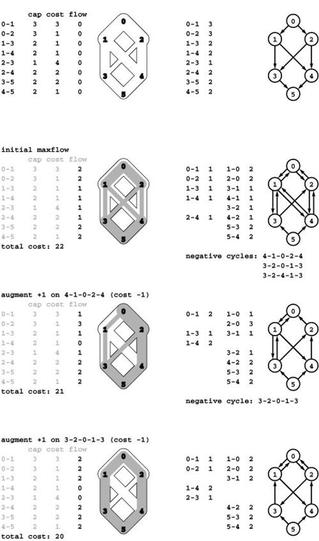
Each of the flows depicted here is a maxflow for the flow network depicted at the top, but only the one at the bottom is a mincost maxflow. To find it, we start with any maxflow and augment flow around negative cycles. The initial maxflow (second from top) has a cost of 22, which is not a min-cost maxflow because the residual network (shown at right) has three negative cycles. In this example, we augment along 4-1-0-2-4 to get a maxflow of cost 21 (third from top), which still has one negative cycle. Augmenting along that cycle gives a mincost flow (bottom). Note that augmenting along 3-2-4-1-3 in the first step would have brought us to the mincost flow in one step.
Program 22.9 Cycle canceling
This class solves the mincost-maxflow problem by canceling negative-cost cycles. It uses MAXFLOW to find a maxflow and a private member function negcyc (see Exercise 22.108) to find negative cycles. While a negative cycle exists, this code finds one, computes the maximum amount of flow to push through it, and does so. The augment function is the same as in Program 22.3, which was coded (with some foresight!) to work properly when the path is a cycle.
template <class Graph, class Edge> class
MINCOST
{ const Graph &G;
int s, t;
vector<int> wt;
vector <Edge *> st;
int ST(int v) const;
void augment(int, int);
int negcyc(int);
int negcyc();
public:
MINCOST(const Graph &G, int s, int t) : G(G),
s(s), t(t), st(G.V()), wt(G.V())
{ MAXFLOW<Graph, Edge>(G, s, t);
for (int x = negcyc(); x != -1; x = negcyc())
{ augment(x, x); }
}
};
lower cost (in general, we do not know the flow value, so there is some flow left in the dummy edge at the end, which we ignore). As is evident from the figure, some augmenting cycles include the dummy edge and increase flow in the network; others do not include the dummy edge and reduce cost. Eventually, we reach a maxflow; at that point, all the augmenting cycles reduce cost without changing the value of the flow, as when we started with a maxflow.
Technically, using a dummy-flow initialization is neither more nor less generic than using a maxflow initialization for cycle canceling. The former does encompass all augmenting-path maxflow algorithms, but not all maxflows can be computed with an augmenting-path algorithm
Figure 22.42 Cycle canceling without initial maxflow
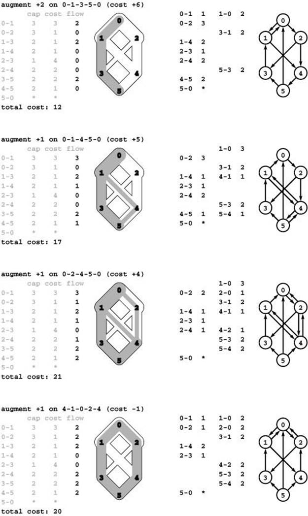
This sequence illustrates the computation of a mincost maxflow from an initially empty flow with the cycle-canceling algorithm by using a dummy edge from sink to source in the residual network with infinite capacity and infinite negative cost. The dummy edge makes any augmenting path from 0 to 5 a negative cycle (but we ignore it when augmenting and computing the cost of the flow). Augmenting along such a path increases the flow, as in augmenting-path algorithms (top three rows). When there are no cycles involving the dummy edge, there are no paths from source to sink in the residual network, so we have a maxflow (third from top). At that point, augmenting along a negative cycle decreases the cost without changing the flow value (bottom). In this example, we compute a maxflow, then decrease its cost; but that need not be the case. For example, the algorithm might have augmented along the negative cycle 1-4-5-3-1 instead of 0-1-4-5-0 in the second step. Since every augmentation either increases the flow or reduces the cost, we always wind up with a mincost maxflow.
(see Exercise 22.40). On the one hand, by using this technique, we may be giving up the benefits of a sophisticated maxflow algorithm; on the other hand, we may be better off reducing costs during the process of building a maxflow. In practice, dummy-flow initialization is widely used because it is so simple to implement.
As for maxflows, the existence of this generic algorithm guarantees that every mincost-flow problem (with capacities and costs that are integers) has a solution where flows are all integers; and the algorithm computes such a solution (see Exercise 22.107). Given this fact, it is easy to establish an upper bound on the amount of time that any cycle-canceling algorithm will require.
Property 22.24 The number of augmenting cycles needed in the generic cycle-canceling algorithm is less than ECM.
Proof: In the worst case, each edge in the initial maxflow has capacity M, cost C, and is filled. Each cycle reduces this cost by at least 1.
Corollary The time required to solve the mincost-flow problem in a sparse network is O(V3CM).
Proof: Immediate by multiplying the worst-case number of augmenting cycles by the worst-case cost of the Bellman–Ford algorithm for finding them (see Property 21.22).
Like that of augmenting-path methods, this running time is extremely pessimistic, as it assumes not only that we have a worst-case situation where we need to use a huge number of cycles to minimize cost, but also that we have another worst-case situation where we have to examine a huge number of edges to find each cycle. In many practical situations, we use relatively few cycles that are relatively easy to find, and the cycle-canceling algorithm is effective.
It is possible to develop a strategy that finds negative-cost cycles and ensures that the number of negative-cost cycles used is less than V E (see reference section). This result is significant because it establishes the fact that the mincost-flow problem is tractable (as are all the problems that reduce to it). However, practitioners typically use implementations that admit a bad worst case (in theory) but use substantially fewer iterations on the problems that arise in practice than predicted by the worst-case bounds.
The mincost-flow problem represents the most general problem-solving model that we have yet examined, so it is perhaps surprising that we can solve it with such a simple implementation. Because of the importance of the model, numerous other implementations of the cycle-canceling method and numerous other different methods have been developed and studied in detail. Program 22.9 is a remarkably simple and effective starting point, but it suffers from two defects that can potentially lead to poor performance. First, each time that we seek a negative cycle, we start from scratch. Can we save intermediate information during the search for one negative cycle that can help us find the next? Second, Program 22.9 just takes the first negative cycle that the Bellman–Ford algorithm finds. Can we direct the search towards negative cycles with particular properties? In Section 22.6, we consider an improved implementation, still generic, that represents a response to both of these questions.
Exercises
22.105 Expand your class for feasible flows from Exercise 22.74 to include costs. Use MINCOST to solves the mincost–feasible-flow problem.
• 22.106 Given a flow network whose edges are not all maximal capacity and cost, give an upper bound better than ECM on the cost of a maxflow.
22.107 Prove that, if all capacities and costs are integers, then the mincostflow problem has a solution where all flow values are integers.
22.108 Implement the negcyc() function for Program 22.9, using the Bellman-Ford algorithm (see Exercise 21.134).
• 22.109 Modify Program 22.9 to initialize with flow in a dummy edge instead of computing a flow.
• 22.110 Give all possible sequences of augmenting cycles that might have been depicted in Program 22.41.
• 22.111 Give all possible sequences of augmenting cycles that might have been depicted in Program 22.42.
22.112 Show, in the style of Program 22.41, the flow and residual networks after each augmentation when you use the cycle-canceling implementation of Program 22.9 to find a mincost flow in the flow network shown in Program 22.10, withcost 2 assigned to 0-2 and 0-3;cost 3 assigned to 2-5 and 3-5; cost 4 assigned to 1-4; and cost 1 assigned to all of the other edges. Assume that the maxflow is computed with the shortest-augmenting-path algorithm.
22.113 Answer Exercise 22.112, but assume that the program is modified to start with a maxflow in a dummy edge from source to sink, as in Program 22.42.
22.114 Extend your solutions to Exercises 22.6 and 22.7 to handle costs in flow networks.
22.115 Extend your solutions to Exercises 22.9 through 22.11 to include costs in the networks. Take each edge’s cost to be roughly proportional to the Euclidean distance between the vertices that the edge connects.
All materials on the site are licensed Creative Commons Attribution-Sharealike 3.0 Unported CC BY-SA 3.0 & GNU Free Documentation License (GFDL)
If you are the copyright holder of any material contained on our site and intend to remove it, please contact our site administrator for approval.
© 2016-2026 All site design rights belong to S.Y.A.