Introduction to Game Design, Prototyping, and Development (2015)
Part I: Game Design and Paper Prototyping
Chapter 11. Math and Game Balance
In this chapter, we explore various systems of probability and randomness and how they relate to paper game technologies. You also learn a little about OpenOffice Calc to help us explore these possibilities.
Following the mathematical explorations (which I promise are as clear and easy to understand as possible), we cover how these systems can be used in both paper and digital games to balance and improve gameplay.
The Meaning of Game Balance
Now that you’ve made your initial game prototype and experimented with it a few times through playtests, you will probably need to balance it as part of your iteration process. Balance is a term that you will often hear when working on games, but it means different things depending on the context.
In a multiplayer game, balance most often means fairness: each player should have an equal chance of winning the game. This is most easily accomplished in symmetric games where each player has the same starting point and abilities. Balancing an asymmetric game is considerably more difficult because player abilities or start positions that may seem balanced could demonstrate a bias toward one player in practice. This is one of the many reasons why playtesting is critically important.
In a single-player game, balance usually means that the game is at an appropriate level of difficulty for the player and the difficulty changes gradually. If a game has a large jump in difficulty at any point, that point becomes a place where the game will tend to lose players. This relates to the discussion of flow as a player-centric design goal in Chapter 8, “Design Goals.”
In this chapter, you learn about several disparate aspects of math that are all part of game design and balance. This includes understanding probability, an exploration of different randomizers for paper games, and the concepts of weighted distribution, permutations, and positive and negative feedback. Throughout this exploration, you use Apache OpenOffice Calc, a spreadsheet program, to better explore and understand the concepts presented. At the end of the chapter, you will see how Calc was used to balance the weapons used in the paper prototype example in Chapter 9, “Paper Prototyping.”
Installing Apache OpenOffice Calc
To start our exploration into game math, I’d like you to download and install Apache OpenOffice. OpenOffice is a suite of applications that is comparable to Microsoft Office but is free and open source. You can download it from http://openoffice.org. The current version as of this writing is 4.1.0. Please visit the website and download Open Office now; we’ll be using it throughout this chapter.1
1 If you are using OS X, it may not allow you to run the OpenOffice app because it was not downloaded directly from the Apple App Store. If this is the case, you should read the support article for Apple Gatekeeper at http://support.apple.com/kb/HT5290 or read the OpenOffice Install Guide at http://www.openoffice.org/download/common/instructions.html.
Note
For this book, I have chosen to use OpenOffice Calc because it is free, cross-platform, and easily available. Many other spreadsheet programs have the same capabilities as Calc (e.g., Microsoft Excel, Google Docs Spreadsheet, and LibreOffice Calc Spreadsheet), but each program is subtly different from the others, so attempting to follow the directions in this chapter in an application other than OpenOffice Calc may lead to frustration.
For some of the things that we’ll be doing in this chapter, a spreadsheet program like Calc isn’t strictly necessary—you could get the same results with a piece of scratch paper and a calculator—however, I feel it’s important to introduce spreadsheets as an aspect of game balance for a few reasons:
![]() A spreadsheet can help you quickly grasp gestalt information from numerical data. In Chapter 9, I presented you with several different weapons that each had different stats. At the end of this chapter, we will recreate the process that I went through to balance those weapons to each other, contrasting weapon stats that I created initially based on gut feeling with those that I refined through use of a spreadsheet.
A spreadsheet can help you quickly grasp gestalt information from numerical data. In Chapter 9, I presented you with several different weapons that each had different stats. At the end of this chapter, we will recreate the process that I went through to balance those weapons to each other, contrasting weapon stats that I created initially based on gut feeling with those that I refined through use of a spreadsheet.
![]() Charts and data can often be used to convince nondesigners of the validity of a game design decision that you have made. To develop a game, you will often be working with many different people, some of whom will prefer to see numbers behind decisions rather than instinct. That doesn’t mean that you should always make decisions with numbers, I just want you to be able to do so if it’s necessary.
Charts and data can often be used to convince nondesigners of the validity of a game design decision that you have made. To develop a game, you will often be working with many different people, some of whom will prefer to see numbers behind decisions rather than instinct. That doesn’t mean that you should always make decisions with numbers, I just want you to be able to do so if it’s necessary.
![]() Many professional game designers work with spreadsheets on a daily basis, but I have seen very few game design programs that teach students anything about how to use them. In addition, the classes at universities that do cover spreadsheet use tend to be more interested in business or accounting than game balance, and therefore focus on different spreadsheet capabilities than I have found useful in my work.
Many professional game designers work with spreadsheets on a daily basis, but I have seen very few game design programs that teach students anything about how to use them. In addition, the classes at universities that do cover spreadsheet use tend to be more interested in business or accounting than game balance, and therefore focus on different spreadsheet capabilities than I have found useful in my work.
As with all aspects of game development, the process of building a spreadsheet is an iterative and somewhat messy process. Rather than show you perfect examples of making spreadsheets from start to finish with every little thing planned ahead of time, the tutorials in this chapter are designed to demonstrate not only the steps to make a spreadsheet but also a realistic iterative process of both building and planning the spreadsheet.
Examining Dice Probability with Calc
A large portion of game math comes down to probability, so it’s critical that you understand a little about how probability and chance work. We’ll start by using OpenOffice Calc to help us understand the probability distribution of rolling various numbers using two six-sided dice (2d6).
On a single roll of a single six-sided die (1d6), you will have any even chance of getting a 1, 2, 3, 4, 5, or 6. That’s pretty obvious. However, things get much more interesting when you’re talking about adding the results of two dice together. If you roll 2d6, then there are 36 different possibilities for the outcome, all of which are shown here:
Die A: 1 2 3 4 5 6 1 2 3 4 5 6 1 2 3 4 5 6 1 2 3 4 5 6 1 2 3 4 5 6 1 2 3 4 5 6
Die B: 1 1 1 1 1 1 2 2 2 2 2 2 3 3 3 3 3 3 4 4 4 4 4 4 5 5 5 5 5 5 6 6 6 6 6 6
It’s certainly possible to write all of these by hand, but I’d like you to learn how to use Calc to do it as an introduction to using a spreadsheet to aid in game balance. Open OpenOffice and create a new Spreadsheet. (Doing so will open the Calc part of OpenOffice.) You should see a new document like the one shown in Figure 11.1.
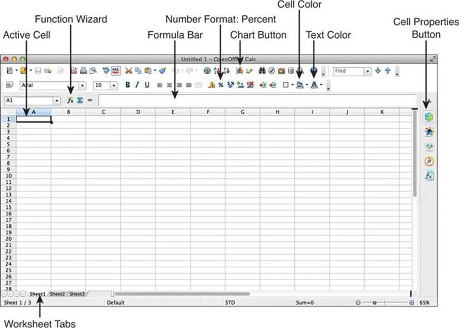
Figure 11.1 A new OpenOffice Calc spreadsheet showing important parts of the interface
Getting Started with Calc
The cells in a spreadsheet are each named with a column letter and a row number. The top-left cell in the spreadsheet is A1. In Figure 11.1, cell A1 is highlighted with a black border and a small black box in its bottom-right corner, showing that it is the Active Cell.
The directions that follow will show you how to get started using Calc:
1. Select cell A1 in OpenOffice by clicking it.
2. Type the number 1 on your keyboard and press Return. A1 will now hold the value 1.
3. Click in cell B1 and type =A1+1 and press Return. This creates a formula in B2 that will constantly calculate its value based on A1. All formulas start with an =. You’ll see that the value of B1 is now 2 (the number you get when you add 1 to the value in A1). If you change the value in A1, B1 will automatically update.
4. Click B1 and copy the cell (Choose Edit > Copy from the menu bar or Command-C on an OS X keyboard or Control+C on a PC keyboard).
5. Hold Shift on the keyboard and Shift-click cell K1. This will highlight the cells from B1 to K1.
6. Paste the formula from B1 into the highlighted cells (Edit > Paste from the menu bar, Command-V on OS X, or Ctrl+V on PC). This will paste the formula that you copied from B1 into the cells from B1 to K1 (that is, the formula =A1+1).
Note
Because the cell reference A1 in the formula is a relative reference, it will update based on the position of the new cell into which it has been pasted. In other words, the formula in K1 will be =J1+1 because J1 is one cell to the left of K1 just as A1 was one to the left of B1.
As a relative reference in the formula of cell B1 (=A1+1), A1 is storing the position of the cell relative to B1 rather than the specific cell location A1. To create an absolute reference (that is, a cell reference that will not change if the formula is copied to another cell), put a $(dollar sign) in front of both the column (A) and row (1). This would give you the formula =$A$1+1 that contains an absolute reference to cell A1. You can also make just the column or row absolute by putting the $ in front of one or the other instead of both.
Creating a Row of Numbers from 1 to 36
The preceding instructions should leave you with the numbers 1 through 11 in the cells A1:K1 (in other words, the cells from A1 to K1; the colon is used to define a range between the two listed cells). Next, we will extend the numbers to count all the way from 1 to 36 (for the 36 possible die rolls):
1. Click B1 to select it.
2. Another way that you can copy the contents of a single cell over a large range is to use the black square in the lower-right corner of a selected cell (which you can see at the lower-right corner of cell A1 in Figure 11.1). Click and drag the black square from the corner of B1 to the right until you have highlighted cells B1:AJ1. When you release the mouse button, you will now see that A1:AJ1 are filled with the series of numbers from 1 to 36.
Setting Column Widths
This has filled the cells A1:AJ1 with the correct data, however these 36 columns are much wider than they actually need to be. We’ll now narrow them to a more appropriate width:
1. Click cell A1.
2. On your keyboard, hold Shift and Command (on Windows, Shift and Control) and press the right-arrow key. This will select all of the cells from A1:AJ1. When holding the Command key, pressing any of the arrow keys will cause the cell highlight to jump to the last filled cell in that direction before an empty cell.
3. From the menu bar, choose Format > Column > Optimal Width. This will open a small dialog box asking you the amount of padding you would like to have (that is, extra space between each column). Leave it set to 0.1" and click the OK button. The columns A through AJ will now narrow to hold their numbers plus 0.1" of extra space. This should make it much easier to fit all of them on your screen at once.
Another way to set column width is to position your mouse directly above the border between two column headings (as is shown in Figure 11.2) and click and drag the border left or right. This will shrink or expand the width of the column. Release the mouse button to set the column to the new width.
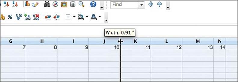
Figure 11.2 Adjusting the column width OpenOffice Calc using the mouse
If you have multiple columns selected (which will highlight them blue as they are in Figure 11.2), this will allow you to set the width of all of them to the same value, but you must select the entire column, not just cells within the column (to do so, click the A column heading and then Shift-click the AJ column heading). Double-clicking the border at the right of a column will set it to the optimal width.
Making the Row for Die A
Now, we have a series of numbers, but what we really want is two rows like those for Die A and Die B that were listed earlier in this chapter. We can achieve this with some simple formulas:
1. Click A2 to select it.
2. Click the Function Wizard button shown in Figure 11.1. This will bring up Calc’s Function Wizard, a dialog box listing all the functions available in Calc.
3. Scroll through the functions to find MOD and click it. The Function Wizard gives you a brief description of the MOD() function, but this description lacks a lot of key information.
4. Click the Help button in the dialog box and then type MOD in the search box and press Return (Enter on PC) to cause the help file to display more information about how MOD works. As the Help states, MOD() returns the remainder when one integer is divided by another. This means that MOD(5;3) would return the value 2 (which is the remainder of 5/3). MOD(6;3) would return 0 because there is no remainder when 6 is divided by 3.
5. Close the Help window, and switch back to the Calc program if necessary.
6. Type =MOD(A1;6) into the Formula field of the Function Wizard. You should see the Result field update to show 1 (the remainder when 1 is divided by 6).
7. Click the OK button in the Function Wizard. This will enter the function from the Function Wizard into cell A2.
8. Copy cell A2 and paste it into cells A2:AJ2 (the colon [:] denotes the range of cells from A2 to AJ2). This will give you the numbers 1 2 3 4 5 0 repeated six times across cells A2:AJ2. Because the reference to A1 in the formula is a relative reference, each cell from A2:AJ2 is taking the value of the cell directly above it and modding it by 6 (i.e., finding the remainder of that value divided by 6).
The results of this formula are very close to what we wanted for Die A. It gives us the numbers 1 2 3 4 5 0 repeating, but we wanted the numbers 1 2 3 4 5 6, so we’ll need to iterate a bit.
Adjusting the Mod Formula
We need to fix two issues through modification to the formulae in A2:AJ2. First, the lowest number should be in columns A, F, L, and so on; and second, the numbers should range from 1 to 6, not 0 to 5. Both of these can be fixed by simple adjustments:
1. Select cell A1 and change its value from 1 to 0. This will cascade through the formulae in B1:AJ1 and give you a series of numbers on row 1 from 0 to 35. Now, the formula in A2 returns 0 (the remainder when 0 is divided by 6), and the numbers in A2:AJ2 will be six series of 0 1 2 3 4 5, which fixes the first issue.
2. To fix the second issue, select A2 and change the formula in A2 to =MOD(A1;6)+1. This will simply add one to the result of the previous formula, which increases the formula result in A2 from 0 to 1. This may seem like we’ve gone in a circle, but once you complete step 3, you’ll see the reason for doing so.
3. Copy A2 and paste it over A2:AJ2. Now, the row for Die A is complete and you have six series of the numbers 1 2 3 4 5 6. The mod values still range from 0 to 5, but now they are in the correct order, and adding 1 to them has generated the numbers that we wanted for Die A.
Making the Row for Die B
The row for Die B includes six repetitions of each number on the die. To accomplish this, we will use the division and floor functions in Calc. Divisions works as you would expect it to (for example, =3/2 will return the result 1.5), however, floor may be a function that you have not encountered before.
1. Select cell A3.
2. Click the Function Wizard button and scroll through the list of functions to find FLOOR. As the Function Wizard shows, FLOOR is used to round decimal numbers to integers, but FLOOR always rounds down. For example, =FLOOR(5.1;1) returns 5 and =FLOOR(5.9;1) also returns 5. The second argument to the FLOOR function (i.e., the ;1 in the preceding examples) sets the significance of the floor. To floor to a whole integer, this argument should always be 1.
3. Enter =FLOOR(A1/6;1) into the Formula field. You will see that the Result field updates to show a result of 0.
4. As was needed with the Die A row, we must add one to the result of the formula. Change the formula to =FLOOR(A1/6;1)+1, and you will see that the result is now 1.
5. Click OK to close the Function Wizard.
6. Copy the contents of A3 and paste them into A3:AJ3.
Your spreadsheet should now look like the top image in Figure 11.3. However, it would be much easier to understand if it were labeled as is shown in the bottom image of Figure 11.3.
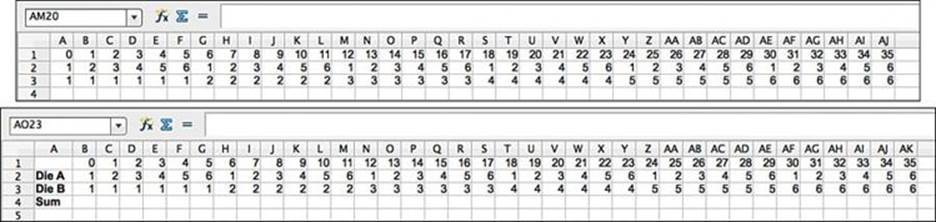
Figure 11.3 Adding clarity with labels
Adding Clarity with Labels
To add the labels shown in the second image of Figure 11.3, you will need to insert a new column to the left of column A:
1. Right-click on any cell in column A and choose Insert from the menu. If you’re on OS X and don’t have a right-click button, you can Control-click. See the section “Right-Click on OS X” in Appendix B, “Useful Concepts,” for more information.
2. From the dialog box that appears, choose Entire column and click OK. This will place a new column A to the left of the existing columns. Note that all of the functions update properly and none of your data or formulae are damaged.
3. Click on the new, empty cell A2 and enter Die A. This won’t fit in the narrow column, but you can easily adjust a column width while typing by holding the Option key (the Alt key on PC) and pressing the right- and left-arrow keys.
4. Enter Die B into A3. Then select A2:A3 and make them bold by either pressing Command-B (Ctrl+B on PC) or clicking the B formatting button above the function bar.
5. Type Sum in A4 and make it bold as well. Your spreadsheet should now look like the second image in Figure 11.3.
Summing the Results of the Two Dice
Another formula will allow you to sum the results of the two dice.
1. Click B4 and enter the formula =SUM(B2;B3), which will sum the values in the cells from B2 to B3 (the formula =B2+B3 would also work equally well). This will put the value 2 into B4.
2. Copy B4 and paste it into B4:AK4. Now, row 4 shows the results of all 36 possible rolls of 2d6.
Counting the Sums of Die Rolls
Row 4 now shows all the results of the 36 possible rolls of 2d6. However, although the data is there, it is still not very easy to interpret it. This is where we can really use the strength of a spreadsheet. To start the data interpretation, we’ll create formulae to count the occurrences of each sum (that is, count how many times we roll a 7 on 2d6):
1. Select cells A7:A17 and from the menu bar choose Edit > Fill > Series. This allows you to fill cells with a series of numbers.
2. Set the Direction to Down, the Start value to 2, and the End value to 12 with an increment of 1.
3. Click OK. This will fill A7:A17 with the numbers from 2 to 12.
4. Select cell B7 and type =COUNTIF( but don’t press the Return or Enter key.
5. Use your mouse to click and drag from B4 to AK4. This will draw a box around B4:AK4 and enter B4:AK4 into your in-progress formula.
6. Type ;.
7. Click A7. This will enter A7 into the formula. At this point, the entire formula should be =COUNTIF(B4:AK4;A7).
8. Type ) and press Return (Windows, Enter). Now, the formula in B7 will be =COUNTIF(B4:AK4;A7).
The COUNTIF function counts the number of times within a series of cells that a certain criterion is met. In cell B7, the COUNTIF function looks at all the cells B4:AK4 and counts the number of times that the number 2 occurs (because 2 is the number in A7).
Next, you will want to extend this from just counting the number of twos to counting the number of rolls of all numbers from 2 to 12:
1. Copy the formula from B7 and paste it into B7:B17.
You will notice that this doesn’t work properly. The counts for all the numbers other than two are 0. Let’s explore why this is happening.
2. Select cell B7 and then click once in the formula bar. This will highlight all of the cells that are used in the calculation of the formula in cell B7.
3. Press the Esc (Escape) key. This is a critical step because it returns you from the cell-editing mode. If you were to click another cell without pressing Esc first, that cell’s reference would be entered into the formula. See the following warning for more information.
Warning
Exiting Formula Editing When working in Calc, you need to press either Return or Esc (Enter or Esc on PC) to exit from editing a formula. Return or Enter will accept the changes that you have made, and Escape will cancel them. If you don’t properly exit from formula editing, any cell you click will be added to the formula (which you don’t want to do accidentally). If this does happen to you, you can press Esc to exit editing without changing the actual formula.
4. Select cell B8 and click once in the formula bar. Now, you should see the problem with the formula in B8. Instead of counting the occurrence of threes in B4:AK4, it is looking for threes in B5:AK5. This is a result of the automatic updating of relative references that was covered earlier in this chapter. Because B8 is one cell lower than B7, all of the references in B8 were updated to be one cell lower. This update of the relative reference is correct for the second argument in the formula (i.e., B8 should be looking for the number in A8 and not A7), but needs to be fixed for the first argument.
5. Press Esc to exit from editing B8.
6. Select B7 and change the formula to =COUNTIF(B$4:AK$4;A7).
7. Copy the formula from B7 and paste it into B7:B17. Now you will see that the numbers update correctly, and each formula in B7:B17 properly queries the cells B$4:AK$4.
Charting the Results
Now, the cells B7:B17 show you the data we wanted. Across the 36 possible rolls of 2d6, there are six possible ways to roll a 7 but only one way to roll a 2 or a 12. This information can be read in the numbers in the cells, but this kind of thing is much easier to understand in a chart:
1. Select cells A7:B17.
2. Click the Chart button (shown in Figure 11.1). This will bring up the Chart Wizard and show you an unrefined version of the chart.
3. The chart type should already be set to Column by default.
4. On the left side of the Chart Wizard, click 2. Data Range and choose the options Data in Columns and First column as label. This will remove the first column (the numbers 2-12) from the chart itself and make them instead the labels at the bottom of the chart.
5. Click 4. Chart Elements and deselect Display Legend. This will remove the legend that had contained Column B from the right side of the chart.
6. Click Finish, and you’ll have a nice chart of the 2d6 data as shown in Figure 11.4. If you click something other than the chart and then click the chart again, you can move it to another location.
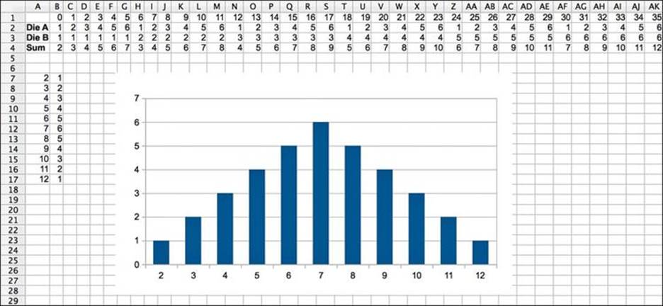
Figure 11.4 A probability distribution chart for 2d6
I know that this was a pretty exhausting way to get this data, but I wanted to introduce you to Calc because it can be an extremely important tool in helping you to balance your games.
The Math of Probability
At this point, you are probably thinking that there must be an easier way to learn about the probability of rolling dice than just enumerating all of the possibilities. Happily, there is an entire branch of mathematics that deals with probability, and this section of the chapter will cover several of the rules that it has taught us.
First, let’s try to determine how many possible different combinations there can be if you roll 2d6. Because there are two dice, and each has 6 possibilities, there are 6 x 6 = 36 different possible rolls of the 2 dice. For 3d6, there are 6 x 6 x 6 = 216, or 63 different combinations. For 8d6, there are 68 = 1,679,616 possibilities! This means that we would require a ridiculously large spreadsheet to calculate the distribution of results from 8d6 if we used the enumeration method that we employed for 2d6.
In The Art of Game Design, Jesse Schell presents “Ten Rules of Probability Every Game Designer Should Know,”2 which I have paraphrased here:
2 Schell, The Art of Game Design, 155-163.
![]() Rule 1: Fractions are decimals are percents: Fractions, decimals, and percents are interchangeable, and you’ll often find yourself switching between them when dealing with probability. For instance, the chance of rolling a 1 on 1d20 is 1/20 or 0.05/1 or 5%. To convert from one to the other, follow these guidelines:
Rule 1: Fractions are decimals are percents: Fractions, decimals, and percents are interchangeable, and you’ll often find yourself switching between them when dealing with probability. For instance, the chance of rolling a 1 on 1d20 is 1/20 or 0.05/1 or 5%. To convert from one to the other, follow these guidelines:
![]() Fraction to Decimal: Type the fraction into a calculator. (Typing 1 ÷ 20 = will give you the result 0.05.)
Fraction to Decimal: Type the fraction into a calculator. (Typing 1 ÷ 20 = will give you the result 0.05.)
![]() Percent to Decimal: Divide by 100 (5% = 5 / 100 = 0.05).
Percent to Decimal: Divide by 100 (5% = 5 / 100 = 0.05).
![]() Decimal to Percent: Multiply by 100 (0.05 = (0.05 * 100)% = 5%).
Decimal to Percent: Multiply by 100 (0.05 = (0.05 * 100)% = 5%).
![]() Anything to Fraction: This is pretty difficult; there’s often no easy way to convert a decimal or percent to a fraction except for the few equivalencies that most people know (e.g., 0.5 = 50% = 1/2, 0.25 = 1/4).
Anything to Fraction: This is pretty difficult; there’s often no easy way to convert a decimal or percent to a fraction except for the few equivalencies that most people know (e.g., 0.5 = 50% = 1/2, 0.25 = 1/4).
![]() Rule 2: Probabilities range from 0 to 1 (which is equivalent to 0% to 100% and 0/1 to 1/1): There can never be less than a 0% chance or higher than a 100% chance of something happening.
Rule 2: Probabilities range from 0 to 1 (which is equivalent to 0% to 100% and 0/1 to 1/1): There can never be less than a 0% chance or higher than a 100% chance of something happening.
![]() Rule 3: Probability is “sought outcomes” divided by “possible outcomes”: If you roll 1d6 and want to get a 6, that means that there is 1 sought outcome (the 6) and 6 possible outcomes (1, 2, 3, 4, 5, or 6). The probability of rolling a 6 is 1/6 (which is roughly equal to 0.16666 or about 17%). There are 13 spades in a regular deck of 52 playing cards, so if you pick one random card, the chance of it being a spade is 13/52 (0.25 or 25%).
Rule 3: Probability is “sought outcomes” divided by “possible outcomes”: If you roll 1d6 and want to get a 6, that means that there is 1 sought outcome (the 6) and 6 possible outcomes (1, 2, 3, 4, 5, or 6). The probability of rolling a 6 is 1/6 (which is roughly equal to 0.16666 or about 17%). There are 13 spades in a regular deck of 52 playing cards, so if you pick one random card, the chance of it being a spade is 13/52 (0.25 or 25%).
![]() Rule 4: Enumeration can solve difficult mathematical problems: If you have a very low number of possible outcomes, enumerating all of them can work fine, as you saw in the 2d6 example in Calc. If you have a larger number (something like 10d6, which has 60,466,176 possible rolls), you could write a computer program to enumerate them. Once you’ve gotten some programming under your belt, you should check out the program to do so that is included in Appendix B.
Rule 4: Enumeration can solve difficult mathematical problems: If you have a very low number of possible outcomes, enumerating all of them can work fine, as you saw in the 2d6 example in Calc. If you have a larger number (something like 10d6, which has 60,466,176 possible rolls), you could write a computer program to enumerate them. Once you’ve gotten some programming under your belt, you should check out the program to do so that is included in Appendix B.
![]() Rule 5: When sought outcomes are mutually exclusive, add their probabilities: Schell’s example of this is figuring the chance of drawing either a face card OR an ace from the deck. There are 12 face cards (3 per suit) and 4 aces in the deck. Aces and face cards are mutually exclusive, meaning that there is no card that is both an ace and a face card. Because of this, if you ask the question, “What is the probability of drawing a face card OR an ace from the deck?” then you can add the two probabilities. 12/52 + 4/52 = 16/52 (0.3077 ≈ 31%). What is the probability of rolling a 1, 2, or 3 on 1d6? 1/6 + 1/6 + 1/6 = 3/6 (0.5 = 50%). Remember, if you use an OR to combine mutually exclusive sought outcomes, you can add their probabilities.
Rule 5: When sought outcomes are mutually exclusive, add their probabilities: Schell’s example of this is figuring the chance of drawing either a face card OR an ace from the deck. There are 12 face cards (3 per suit) and 4 aces in the deck. Aces and face cards are mutually exclusive, meaning that there is no card that is both an ace and a face card. Because of this, if you ask the question, “What is the probability of drawing a face card OR an ace from the deck?” then you can add the two probabilities. 12/52 + 4/52 = 16/52 (0.3077 ≈ 31%). What is the probability of rolling a 1, 2, or 3 on 1d6? 1/6 + 1/6 + 1/6 = 3/6 (0.5 = 50%). Remember, if you use an OR to combine mutually exclusive sought outcomes, you can add their probabilities.
![]() Rule 6: When sought outcomes are not mutually exclusive, multiply their probabilities: If you want to know the probability of choosing a card that is both a face card AND a spade, you can multiply the two probabilities together. There are 13 spades (13/52) and 12 face cards (12/52). Multiplied together, you get the following:
Rule 6: When sought outcomes are not mutually exclusive, multiply their probabilities: If you want to know the probability of choosing a card that is both a face card AND a spade, you can multiply the two probabilities together. There are 13 spades (13/52) and 12 face cards (12/52). Multiplied together, you get the following:
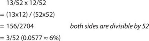
We know this is correct because there are actually 3 spades that are face cards in the deck (which is 3 out of 52). Another example would be the probability of rolling a 1 on 1d6 AND a 1 on another 1d6. This would be 1/6 x 1/6 = 1/36 (0.0278 ≈ 3%), and as we saw in the enumerated example in Calc, there is exactly a 1/36 chance of getting a 1 on both dice when you roll 2d6.
Remember, if you use an AND to combine non-mutually exclusive sought outcomes, you can multiply their probabilities.
Corollary: When sought outcomes are independent, multiply their probabilities: If two actions are completely independent of each other (which is a subset of their not being mutually exclusive), the probability of them both happening is the multiplication of their individual probabilities. For instance, the probability of rolling a 6 on 1d6 is 1/6. The two dice in a 2d6 roll are completely independent of each other, so the probability of getting 6 on both dice is the multiple of the two independent probabilities ( 1/6 x 1/6 = 1/36 ) as we saw in our enumerated example in Calc. The probability of getting a 6 on 2d6 AND getting heads on two coin tosses is ( 1/6 x 1/6 x 1/2 x 1/2 = 1/184 ).
![]() Rule 7: One minus “does” = “doesn’t”: The probability of something happening is 1 minus the probability of it not happening. For instance the chance of rolling a 1 on 1d6 is 1/6, as you know. This means that the chance of not rolling a 1 on 1d6 is 1 - 1/6 = 5/6 (0.8333 ≈ 83%). This is useful because it is sometimes easier to figure out the chance of something not happening than something happening.
Rule 7: One minus “does” = “doesn’t”: The probability of something happening is 1 minus the probability of it not happening. For instance the chance of rolling a 1 on 1d6 is 1/6, as you know. This means that the chance of not rolling a 1 on 1d6 is 1 - 1/6 = 5/6 (0.8333 ≈ 83%). This is useful because it is sometimes easier to figure out the chance of something not happening than something happening.
For example, what if you wanted to calculate the odds of rolling a 6 on at least one die when you roll 2d6? If we enumerate, we’ll find that the answer is 11/36 (the sought outcomes being 6_x, x_6, AND 6_6 where the x could be any number other than 6). You can also count the number of columns with at least one 6 in them in the Calc chart we made. However, we can also use rules 5, 6, and 7 to figure this out mathematically.
The possibility of rolling a 6 on 1d6 is 1/6. The possibility of rolling a non-6 on 1d6 is 5/6, so the possibility of rolling 6 AND a non-6 (6_x) is 1/6 x 5/6 = 5/36. (Remember, AND means multiply from Rule 6.) Because this can be accomplished by either rolling 6_x OR x_6, we add those two possibilities together: 5/36 + 5/36 = 10/36. (Rule 5: OR means add.)
The possibility of rolling a 6 AND a 6 (6_6) is 1/6 x 1/6 = 1/36. Because this is another possible mutually exclusive case from 6_x OR x_6, they can be added together: 5/36 + 5/36 + 1/36 = 11/36 (0.3055 ≈ 31%).
This got complicated pretty quickly, but we can actually use Rule 7 to simplify it. If you reverse the problem and look for the chance of not getting a 6 in two rolls, that can be restated “What is the chance of getting a non-6 on the first roll AND a non-6 on the second roll?” These two sought possibilities are not mutually exclusive, so you can multiply them! So, the chance of getting a non-6 on both rolls is just 5/6 x 5/6 or 25/36. 1 - 25/36 = 11/36, which is pretty awesome and a lot easier to figure out!
Now, what if you were to roll 4d6 and sought at least one 6? This is now simply:
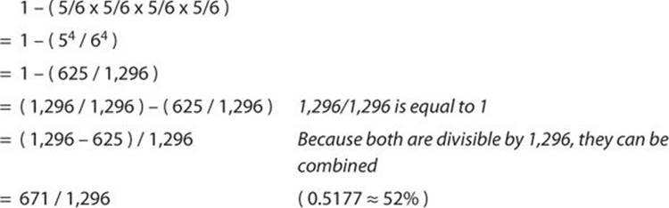
There is about a 52% chance of rolling at least one 6 on 4d6.
![]() Rule 8: The sum of multiple dice is not a linear distribution: As we saw in the enumerated Calc example of 2d6, though each of the individual dice has a linear distribution. That is, each number 1-6 has an equal chance of happening on 1d6, and when you sum multiple dice together, you get a weighted distribution of probability. It gets even more complex with more than two dice, as shown in Figure 11.5.
Rule 8: The sum of multiple dice is not a linear distribution: As we saw in the enumerated Calc example of 2d6, though each of the individual dice has a linear distribution. That is, each number 1-6 has an equal chance of happening on 1d6, and when you sum multiple dice together, you get a weighted distribution of probability. It gets even more complex with more than two dice, as shown in Figure 11.5.
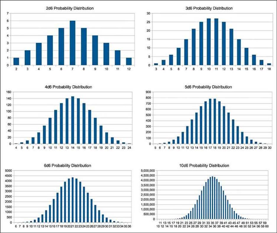
Figure 11.5 Probability distribution for 2d6, 3d6, 4d6, 5d6, 6d6, and 10d6
As you can see in the figure, the more dice you add, the more severe the bias is toward the average sum of the dice. In fact, with 10d6, you have a 1/60,466,176 chance of rolling all 6s, but a 4,395,456/60,466,176 (0.0727 ≈ 7%) chance of rolling exactly 35 or a 41,539,796/60,466,176 ( 0.6869922781 ≈ 69% ) chance of rolling a number from 30 to 40. There are a couple of complex math papers about how to calculate these values with a formula, but I followed Rule 4 and wrote a program to do so.
As a game designer, it’s not important for you to understand the exact numbers of these probability distributions. The thing that it is very important for you to remember is this: The more dice you have the player roll, the more likely they are to get a number near the average.
![]() Rule 9: Theoretical versus practical probability: In addition to the theoretical probabilities that we’ve been talking about, it is sometimes easier to approach probability from a more practical perspective, or to put this another way, the results of rolling actual dice don’t always match the theoretical peredictions. There are both digital and analog ways in which this can be done.
Rule 9: Theoretical versus practical probability: In addition to the theoretical probabilities that we’ve been talking about, it is sometimes easier to approach probability from a more practical perspective, or to put this another way, the results of rolling actual dice don’t always match the theoretical peredictions. There are both digital and analog ways in which this can be done.
Digitally, you could write a simple computer program to do millions of trials and determine the outcome. This is often called the Monte Carlo method, and it is actually used by several of the best artificial intelligences that have been devised to play Chess and Go. Go is so complex that the best a computer can do is to calculate the results of millions of random plays by both the computer and its human opponent and determine the play that statistically leads to the best outcome for it. This can also be used to determine the answers to what would be very challenging theoretical problems. Schell’s example of this is a computer program that could rapidly simulate millions of rolls of the dice in Monopoly and let the programmer know which spaces on the board players were most likely to land on.
Another aspect of this rule is that not all dice are created equal. For instance, if you wanted to publish a board game and were looking for a manufacturer for your dice, it would be very worthwhile to get a couple dice from each potential manufacturer and roll each of them a couple hundred times, recording the result each time. This might take an hour or more to accomplish, but it would tell you whether the dice from the manufacturer were properly weighted or if they would instead roll a certain number more often than the others.
![]() Rule 10: Phone a friend: Nearly all college students who major in computer science or math will have to take a probability class or two as part of their studies. If you run into a difficult probability problem that you can’t figure out on your own, try asking one of them. In fact, according to Schell, the study of probability began in 1654 when the Chevalier de Méré couldn’t figure out why he seemed to have a better than even chance of rolling at least one 6 on four rolls of 1d6 but seemed to have a less than even chance of rolling at least one 12 on 24 rolls of 2d6. The Chevalier asked his friend Blaise Pascal for help. Pascal wrote to his father’s friend Pierre de Fermat, and their conversation became the basis for probability studies.3 Now, using the 10 rules here, you should be able to figure out why.
Rule 10: Phone a friend: Nearly all college students who major in computer science or math will have to take a probability class or two as part of their studies. If you run into a difficult probability problem that you can’t figure out on your own, try asking one of them. In fact, according to Schell, the study of probability began in 1654 when the Chevalier de Méré couldn’t figure out why he seemed to have a better than even chance of rolling at least one 6 on four rolls of 1d6 but seemed to have a less than even chance of rolling at least one 12 on 24 rolls of 2d6. The Chevalier asked his friend Blaise Pascal for help. Pascal wrote to his father’s friend Pierre de Fermat, and their conversation became the basis for probability studies.3 Now, using the 10 rules here, you should be able to figure out why.
3 Schell, The Art of Game Design, 154.
In Appendix B, I have included a Unity program that will calculate the distribution of rolls for any number of dice with any number of sides (as long as you have enough time to wait for it to calculate).
Randomizer Technologies in Paper Games
Some of the most common randomizers used in paper games include dice, spinners, and decks of cards.
Dice
We’ve already covered a lot of information about dice in this chapter. The important elements are as follows:
![]() A single die generates randomness with a linear probability distribution.
A single die generates randomness with a linear probability distribution.
![]() The more dice you add together, the more the result is biased toward the average (and away from a linear distribution).
The more dice you add together, the more the result is biased toward the average (and away from a linear distribution).
![]() Standard die sizes include: d4, d6, d8, d10, d12, and d20. Commonly available packs of dice for gaming usually include 1d4, 2d6, 1d8, 2d10, 1d12, and 1d20.
Standard die sizes include: d4, d6, d8, d10, d12, and d20. Commonly available packs of dice for gaming usually include 1d4, 2d6, 1d8, 2d10, 1d12, and 1d20.
![]() 2d10 are sometimes called percentile dice because one will be used for the 1s place (marked with the numbers from 0-9) and the other for the 10s place (marked with the multiples of 10 from 00-90), giving an even distribution of the numbers from 00 to 99 (where a roll of 0 and 00 is usually counted as 100%).
2d10 are sometimes called percentile dice because one will be used for the 1s place (marked with the numbers from 0-9) and the other for the 10s place (marked with the multiples of 10 from 00-90), giving an even distribution of the numbers from 00 to 99 (where a roll of 0 and 00 is usually counted as 100%).
Spinners
There are a couple of different kinds of spinners, but all have a rotating element and a still element. In most board games, the spinner is composed of a cardboard base that is divided into sections with a spinning arrow mounted above it (see image A in Figure 11.6). Larger spinners (for example, the wheel from the television show Wheel of Fortune) often have the sections on the spinning wheel and the arrow on the base (see Figure 11.6, image B). As long as players spin the spinner with enough force, a spinner is effectively the same as a die from a probability standpoint.
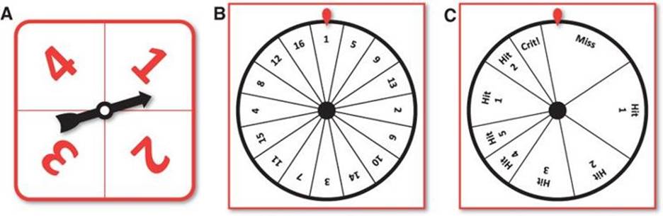
Figure 11.6 Various spinners. In all diagrams, the red elements are static, and the black element rotates.
Spinners are often used in children’s games for two major reasons:
![]() Young children lack the motor control to throw a die within a small area, so they will often accidentally throw dice in a way that they roll off of the gaming table.
Young children lack the motor control to throw a die within a small area, so they will often accidentally throw dice in a way that they roll off of the gaming table.
![]() Spinners are a lot more difficult for young children to swallow.
Spinners are a lot more difficult for young children to swallow.
Though they are less common in games for adults, spinners provide interesting possibilities that are not feasible with dice:
![]() Spinners can be made with any number of slots. However, it is difficult (though not impossible) to construct a die with 3, 7, 13, or 200 sides.
Spinners can be made with any number of slots. However, it is difficult (though not impossible) to construct a die with 3, 7, 13, or 200 sides.
![]() Spinners can be weighted very easily so that not all possibilities have the same chance of happening. Image C of Figure 11.6 shows a hypothetical spinner to be used by a player when attacking. On this spinner, the player would have a 3/16 chance of a Miss, 5/16 chance of Hit 1, 3/16 chance of Hit 2, 2/16 chance of Hit 3, and 1/16 chance of Hit 4, Hit 5, or Crit!
Spinners can be weighted very easily so that not all possibilities have the same chance of happening. Image C of Figure 11.6 shows a hypothetical spinner to be used by a player when attacking. On this spinner, the player would have a 3/16 chance of a Miss, 5/16 chance of Hit 1, 3/16 chance of Hit 2, 2/16 chance of Hit 3, and 1/16 chance of Hit 4, Hit 5, or Crit!
Decks of Cards
A standard deck of playing cards includes 13 cards of 4 different suits and sometimes two jokers (see Figure 11.7). This includes the ranks 1 (also called the Ace) through 10, Jack, Queen, and King in each of the four suits: Clubs, Diamonds, Hearts, and Spades.
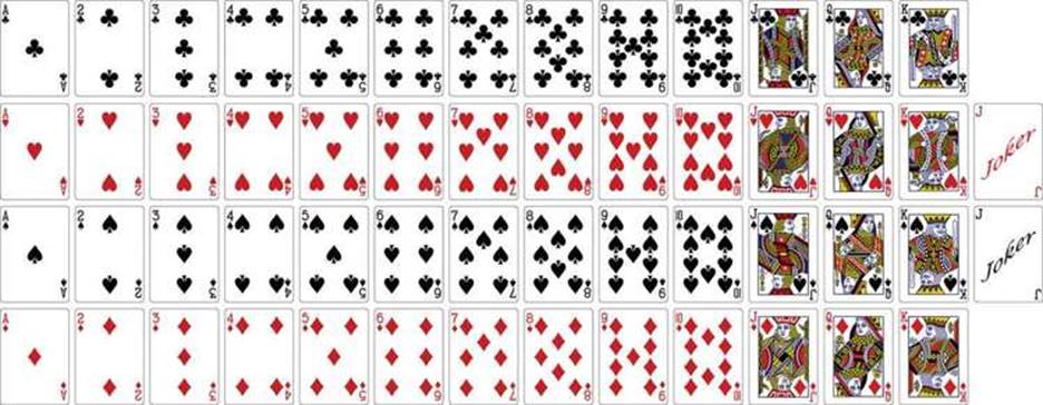
Vectorized Playing Cards 1.3 (http://code.google.com/p/vectorized-playing-cards/) ©2011 - Chris Aguilar Licensed under LGPL 3 - www.gnu.org/copyleft/lesser.html
Figure 11.7 A standard deck of playing cards with two jokers
Playing cards are very popular because of both their compactness and the many different ways that they can be divided.
In a draw of a single card from a deck without Jokers, you have the following probabilities:
![]() Chance of drawing a particular single card: 1/52 (0.0192 ≈ 2%)
Chance of drawing a particular single card: 1/52 (0.0192 ≈ 2%)
![]() Chance of drawing a specific suit: 13/52 = 1/4 (0.25 = 25%)
Chance of drawing a specific suit: 13/52 = 1/4 (0.25 = 25%)
![]() Chance of drawing a face card (J, Q, or K): 12/52 = 3/13 (0.2308 ≈ 23%)
Chance of drawing a face card (J, Q, or K): 12/52 = 3/13 (0.2308 ≈ 23%)
Custom Card Decks
A deck of cards is one of the easiest and most configurable randomizers that can be made for a paper game. You can very easily add or remove copies of a specific card to change the probability of that card appearing in a single draw from the deck. See the section on weighted distributions later in this chapter for more information.
Tips for Making Custom Card Decks
One of the difficulties in making custom cards is getting material for them that you can easily shuffle. 3x5 note cards don’t work particularly well for this, but there are a couple of better options:
![]() Use marker or stickers to modify an existing set of cards. Sharpies work well for this and don’t add thickness to the card like stickers do.
Use marker or stickers to modify an existing set of cards. Sharpies work well for this and don’t add thickness to the card like stickers do.
![]() Buy a deck of card sleeves, and insert a slip of paper along with a regular card into each, as described in Chapter 9.
Buy a deck of card sleeves, and insert a slip of paper along with a regular card into each, as described in Chapter 9.
The key thing you want to avoid when making a deck (or any element of a paper prototype) is putting too much time into any one piece. After you’ve devoted time to making a lot of nice cards (for instance) you may be less willing to remove any of those cards from the prototype or to scrap them and start over.
When to Shuffle a Deck
If you shuffle the entire deck of cards before every draw, then you will have an equal likelihood of drawing any of the cards (just like when you roll a die or use a spinner). However, this isn’t how most people use decks of cards. In general, people will draw until the deck is completely exhausted and then shuffle all the cards. This leads to very different behavior from a deck than from an equivalent die. If you had a deck of six cards numbered 1-6, and you drew every card before reshuffling, you would be guaranteed to see each of the numbers 1-6 once for every six times you drew from the deck. Rolling a die six times will not give you this same consistency. An additional difference is that players could count cards and know which have and have not been drawn thus far, giving them insight into the probability of a certain card being drawn next. For example, if the cards 1, 3, 4, and 5 have been drawn from the six-card deck, there is a 50% chance that the next card will be a 2 and a 50% chance that it will be a 6.
This difference between decks and dice came up in the board game Settlers of Catan where some players got so frustrated at the difference between the theoretical probability of the 2d6 rolls in the game versus the actual numbers that came up in play that the publisher of the game now sells a deck of 36 cards (marked with each of the possible outcomes of 2d6) to replace the dice in play, ensuring that the practical probability experienced in the game is the same as the theoretical probability.
Weighted Distributions
A weighted distribution is one in which some options are more likely to come up than others. Most of the examples that we’ve looked at so far involved linear distributions of random possibilities, but it is a common desire as a designer to want to weight one option more heavily than another. For example, in the board game Small World, the designers wanted an attacker to get a random bonus on her final attack of each turn about half of the time, and they wanted that bonus to range from +1 to +3. To do this, they created a die with these six sides (see Figure 11.8).
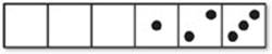
Figure 11.8 The attack bonus die from Small World with weighted bonus distribution
With this die, the chance of getting no bonus is 3/6 = 1/2 (0.5 = 50%), and the chance of getting a bonus of 2 is 1/6 (0.1666 ≈ 17%), so the chance of no bonus is weighted much more heavily than the other three choices.
What if instead, you still wanted the player to get a bonus only half of the time, but you wanted for the bonus of 1 to be three times more likely than the 3, and the 2 to be twice as likely as the 3. This would give us the weighted distribution shown in Figure 11.9.
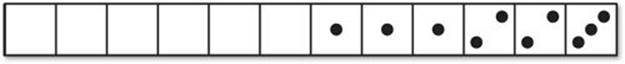
Figure 11.9 Die with 1/2 chance of 0, 1/4 chance of 1, 1/6 chance of 2, and 1/12 chance of 3
Luckily, this adds up to 12 total possible sides for a die (a common die size). However, if it didn’t add up to a common size, you could always create a spinner or a deck of cards with the same probabilities (though the card deck would need to be shuffled each time before drawing a card). It’s also possible to model weighted distributions with randomized outcomes in Calc. Doing so is very similar to how you will deal with random numbers later in Unity and C#.
Weighted Probability in Calc
Weighted probability is commonplace in digital games. For instance, if you wanted an enemy who encounters the player to attack her 40% of the time, adopt a defensive posture 40% of the time, and run away 20% of the time, you could create an array of values [ Attack, Attack, Defend, Defend, Run ]4 and have the enemy’s artificial intelligence code pull a random value from it when the player was first detected.
4 Square brackets ([ ]) are used in C# to define arrays (a group of values), so I’m using them here to group the five possible action values.
Following these steps will give you a Calc worksheet that can be used to randomly select from a series of values. Initially, it will pick a random number between 1 and 12, and once the worksheet is made, you can replace choices in column A with any that you choose.
1. Open a new document in Calc.
2. Fill in everything shown in columns A and B of Figure 11.10 but leave column C empty for now. To right-align the text in column B, select cells B1:B4 and choose Format > Alignment > Right from the Calc menu bar.
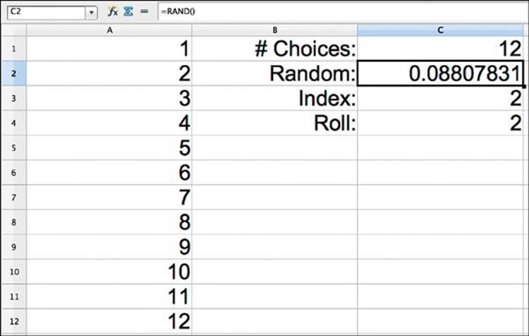
Figure 11.10 OpenOffice Calc table for weighted random number selection
3. Select cell C1 and enter the formula =COUNTIF(A1:A100;"<>"). This will count the number of cells in the range A1:A100 that are not empty (in Calc, <> means “different from,” and not following it with a specified value means “different from nothing”). This gives us the number of valid choices that are listed in column A (we currently have 12).
4. In cell C2 enter the formula =RAND(), which will generate a number from 0 to 1 (including 0, but never actually reaching 1).
5. Select cell C3 and enter the formula =FLOOR(C2*C1;1)+1. The number we’re flooring is the random number between 0 and 0.9999 multiplied by the number of possible choices, which is 12 in this case. This means that we’re flooring numbers between 0 and 11.9999 to give us the integers from 0 to 11. Then we add 1 to the result to give us the integers 1 to 12.
6. In cell C4, enter the formula =INDEX(A1:A100;C3). INDEX() takes a range of values (e.g., A1:A100) and chooses from them based on an index (C3 in this case, which can range from 1 to 12). Now, C4 will choose a random value from the list in column A.
To get a different random value, press F9 on your keyboard. (If you’re on OS X, you probably need to hold the fn key and then press F9.) This will cause Calc to recalculate all formulas on the page (including the RAND() formula) and give you another random number.
You can put either numbers or text into the cells in column A as long as you don’t skip any rows. Try replacing the numbers in cells A1:A12 with the weighted values from Figure 11.9 (that is, [0, 0, 0, 0, 0, 0, 1, 1, 1, 2, 2, 3 ]). If you do so and try recalculating the random value in C3 several times, you will see that zero comes up about half of the time. You can also fill the values A1:A5 with [ Attack, Attack, Defend, Defend, Run ] and see the weighted enemy A1 choice that was used as an example at the beginning of this section.
Permutations
There is a traditional game called Bulls and Cows (see Figure 11.11) that served as the basis for the board game Master Mind (1970 by Mordecai Meirowitz). In this game, each player starts by writing down a secret four-digit code (where each of the digits are different). Players take turns trying to guess their opponent’s code, and the first person to guess correctly wins. When a player guesses, her opponent responds with a number of bulls and a number of cows. The guesser gets a bull for each number she guessed that is in the correct position and a cow for each number that is part of the code but in an incorrect position. In the diagram below, red represents a bull, and white represents a cow.
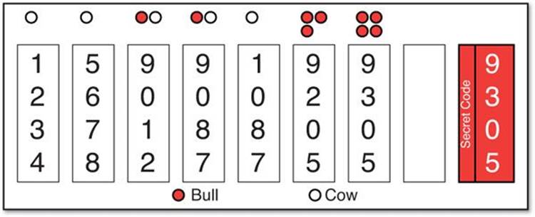
Figure 11.11 An example game of Bulls and Cows
From the perspective of the guesser, the secret code is effectively a series of random choices. Mathematicians call series like these permutations. In Bulls and Cows, the secret code is a permutation of the ten digits 0-9, where four are chosen with no repeating elements. In the game Master Mind, there are eight possible colors, of which four are chosen with no repetition. In both cases, the code is a permutation and not a combination because the positions of the elements matter (9305 is not the same as 3905). A combination is a selection of choices where the position doesn’t matter. For example, 1234, 2341, 3421, 2431, and so on are all the same thing in a combination.
Permutations with Repeating Elements
We’ll start with permutations that allow repetition because the math is a little easier. If there were four digits with repetition allowed, there would be 10,000 possible combinations (the numbers 0000 through 9999). This is easy to see with numbers, but we need a more general way of thinking about it (for cases where there are not exactly 10 choices per slot). Because each digit is independent of the others and each has 10 possible choices, according to probability Rule 6, the probability of getting any one number is 1/10 x 1/10 x 1/10 x 1/10 = 1/10,000. This also tells us that there are 10,000 possible choices for the code (if repetition is allowed).
The general calculation for permutations with repetition allowed is to multiply the number of choices for each slot by each other. With four slots and ten choices each, this is 10 x 10 x 10 x 10 = 10,000. If you were to make the code from six-sided dice instead of digits, then there would be six choices per slot, making 6 x 6 x 6 x 6 = 1296 possible choices.
Permutations with No Repeating Elements
But what about the actual case for Bulls and Cows where you’re not allowed to repeat any digits? It’s actually simpler than you might imagine. Once you’ve used a digit, it’s no longer available. So, for the first slot, you can pick any number from 0-9, but once a digit (e.g., 9) has been chosen for the first slot, there are only 9 choices remaining for the second slot (0-8). This continues for the rest of the slots, so the calculation of possible codes for Bulls and Cows is actually 10 x 9 x 8 x 7 = 5040. Almost half of the possible choices are eliminated by not allowing repeating digits.
Positive and Negative Feedback
One of the most important concepts to understand about game balancing is that of positive and negative feedback. In a game with positive feedback, a player who takes an early lead gains an advantage over the other players and is more likely to win the game. In a game with negativefeedback, the players who are losing have an advantage.
Poker is an excellent example of a game with positive feedback. If a player wins a big pot and has more money than the other players, individual bets matter less to her, and she has more freedom to do things like bluff (because she can afford to lose). However, a player who loses money early in the game and has little left can’t afford to take risks and has less freedom when playing. Monopoly has a strong positive feedback mechanism where the player with the best property consistently gets more money and is able to force other players to sell her their property if they can’t afford the rent when they land on her spaces. Positive feedback is generally frowned upon in multiplayer games, but it can be very good if you want the game to end quickly. Single-player games also often have positive feedback mechanisms to make the player feel increasingly powerful throughout the game.
Mario Kart is a great example of a game with negative feedback in the form of the random items that it awards to players when they drive through item boxes. The player in the lead will usually only get a banana (a largely defensive weapon), a set of three bananas, or a green shell (one of the weakest attacks). A player in last place will often get much more powerful items like a lightning bolt that slows every other player in the race. Negative feedback makes games feel more fair to the players who are not in the lead and generally leads to both longer games and to all players feeling that they have still have a chance of winning even if they’re pretty far behind.
Using Calc to Balance Weapons
Another use of math and programs like OpenOffice Calc in game design is the balance of various weapons or abilities. In this section, we’ll look at the process that went into balancing the weapons for the paper prototype example in Chapter 9. As you saw in Chapter 9, each weapon has values for three things:
![]() The number of shots fired at a time
The number of shots fired at a time
![]() The damage done by each shot
The damage done by each shot
![]() The chance that each shot will hit at a given distance
The chance that each shot will hit at a given distance
As we balance these weapons, we want them to feel roughly equal to each other in power, though we want each weapon to have a distinct personality. For each weapon, this would be as follows:
![]() Pistol: A basic weapon; pretty decent in most situations but doesn’t excel in any
Pistol: A basic weapon; pretty decent in most situations but doesn’t excel in any
![]() Rifle: A good choice for mid and long range
Rifle: A good choice for mid and long range
![]() Shotgun: Deadly up close but its power falls off quickly; only one shot, so a miss really matters
Shotgun: Deadly up close but its power falls off quickly; only one shot, so a miss really matters
![]() Sniper Rifle: Terrible at close range but fantastic at long range
Sniper Rifle: Terrible at close range but fantastic at long range
![]() Machine Gun: Fires many shots, so even if some miss, the others will usually hit; this should feel like the most reliable gun, though not the most powerful
Machine Gun: Fires many shots, so even if some miss, the others will usually hit; this should feel like the most reliable gun, though not the most powerful
Figure 11.12 shows the values for the weapons as I initially imagined they might work. The ToHit value is the minimum roll on 1d6 that would hit at that range. For example, in cell K3, you can see that the ToHit for the pistol at a range of 7 is 4, so if shooting a target 7 spaces away, any of 4 or above would be a hit. This is a 50% chance of hitting on 1d6 (because it would hit on a roll of 4, 5, or 6).
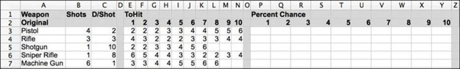
Figure 11.12 Initial values for the weapons balance spreadsheet
Create a new spreadsheet document in Calc and enter all of the data shown in Figure 11.12. To change the background color of a cell, you can use the Cell Color button shown in Figure 11.1.
Determining the Percent Chance for Each Bullet
In the cells under the heading Percent Chance, we want to calculate the chance that each shot of a weapon will hit at a certain distance. To do so, follow these steps.
1. In cell E3, you can see that each shot from a pistol will hit at a distance of 1 if the player rolls a 2 or better on 1d6. This means that it will miss on a 1 and hit on 2, 3, 4, 5, or 6. This is a 5/6 chance (or ≈83%), and we need a formula to calculate this. Looking at probability rule #7, we know that there is a 1/6 chance of it missing (which is the same as the ToHit number minus 1). Select cell P3 and enter the formula =(E3-1)/6. This will cause P3 to display the chance of the pistol missing at a range of one.
2. Using Rule 7 again, we know that 1-miss = hit, so change the formula in P3 to =1-((E3-1)/6). Order of operations works in Calc, so divide operations happen before minus operations. To enforce the order in which I want the operations to occur, I’ve added parentheses. Once you’ve done this, P3 will hold the value 0.8333333.
3. To convert P3 from showing decimal numbers to showing a percentage, click the Number Format: Percent button shown in Figure 11.1. You will also probably want to click the Number Format: Delete Decimal Place button a couple times. It is the button to the right of Number Format: Percent that shows .000 with a red X above it.
4. Copy the formula in P3 and paste it into all the cells in the range P3:Y7. You’ll see that everything works perfectly except for the blank ToHit cells, which now have a percent chance of %117! The formula needs to be altered to ignore blank cells.
5. Select P3 again and change the formula to =IF(E3="";"";1-((E3-1)/6)). The IF statement has three parts, which are divided by semicolons.
![]() E3="": The first part is a question: Is E3 equal to "". That is, is E3 equal to an empty cell.
E3="": The first part is a question: Is E3 equal to "". That is, is E3 equal to an empty cell.
![]() "": The second part is what to put in the cell if the question evaluates to true. That is, if E3 is empty, make cell P3 empty as well.
"": The second part is what to put in the cell if the question evaluates to true. That is, if E3 is empty, make cell P3 empty as well.
![]() 1-((E3-1)/6): The third part is what to put in the cell if the question evaluates to false. (That is, if E3 is not empty, then use the same formula we had before.)
1-((E3-1)/6): The third part is what to put in the cell if the question evaluates to false. (That is, if E3 is not empty, then use the same formula we had before.)
6. Copy the new formula from P3 and paste it into P3:Y7. You will see that the empty cells in the ToHit area now cause empty cells in the Percent Chance area. (For example, L5:N5 are empty, so W5:Y5 are empty as well.) It should now look like the Percent Chance section in Figure 11.13.
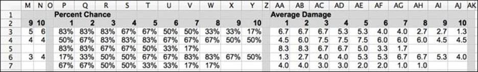
Figure 11.13 The Percent Chance and Average Damage sections of the weapons spreadsheet. You will be making the Average Damage section next. (Note that the spreadsheet has been scrolled to the right to show columns M through AK.)
Calculating Average Damage
The next step in the balancing process is to determine how much average damage each gun will do at a certain distance. Because some guns fire multiple shots and each shot has a certain amount of damage, the average damage will be equal to the number of shots fired * the amount of damage per shot * the chance that each shot will hit:
1. Select cell AA3 and enter the formula =IF(P3="";"";$B3*$C3*P3). Just like in the formula for P3, the IF statement here ensures that only non-empty cells are calculated. The formula includes absolute column references for cells $B3 and $C3 because B3 is the number of shots, and C3 is the damage per shot. We don’t want those references moving to other columns (though we do want them able to move to other rows, so only the column reference is absolute).
2. Copy cell AA3 and paste it into AA3:AJ7. Now your Average Damage section should look like the one shown in Figure 11.13.
Charting the Average Damage
The next important step is to chart the average damage. While it’s possible to look carefully at the numbers and interpret them, it’s much easier to have Calc do the job of charting information, allowing you to visually assess what is going on. Follow these steps to do so:
1. Click and drag to select cells AA3:AJ7.
2. Click the Chart button (see Figure 11.1) to bring up the Chart Wizard. This chart will be a little more complex than the previous one.
3. In step 1. Chart Type, choose Line from the list of chart types. This will give you four options of line charts as icons to the right of the list of cart types.
4. Choose the Lines Only type of line chart, which is the third option.
5. Click 2. Data Range in the list of steps at the left of the Chart Wizard.
6. The data for each weapon is stored in a row, so choose the Data series in rows option. Now, the chart will start to look a little more like you might have expected.
7. To use the names of the weapons as labels, they must be part of the data range of the chart. Change the text in the Data range field to $A$3:$A$7;$AA$3:$AJ$7. This will include the gun names in A3:A7 as the first column of the data range.
8. Check the First column as label option. This will now use the gun names as labels for the five lines in the chart.
9. Click the Finish button to complete the chart.
10. To move the chart when it is selected, move your mouse near the border of the chart, and the mouse icon will change to a hand. Then you can click and drag to move the chart. You can also drag the small green boxes around the border to resize the chart.
You can see the results of the chart in the bottom of Figure 11.14. As you can see, there are some problems with the weapons. Some, like the sniper rifle and shotgun, have personalities as we had hoped (the shotgun is deadly at close range, and the sniper rifle is better at long range), but there are a lot of other problems:
![]() The machine gun is ridiculously weak.
The machine gun is ridiculously weak.
![]() The pistol may be too strong.
The pistol may be too strong.
![]() The rifle is also overly strong compared to the other weapons.
The rifle is also overly strong compared to the other weapons.
In short, the weapons are not balanced well to each other.
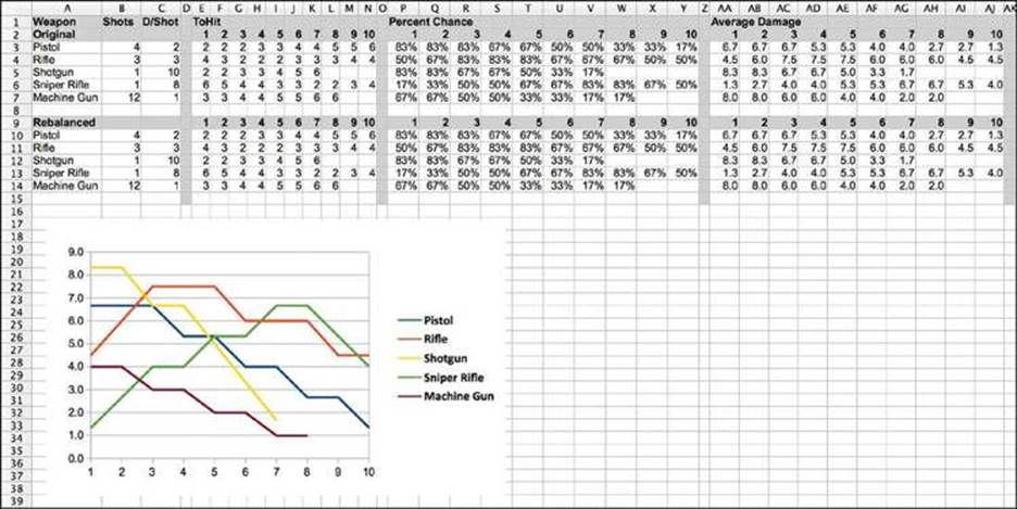
Figure 11.14 The weapon balance at the halfway point showing the chart of initial weapon stats. The Original and Rebalanced sections of the spreadsheet are also shown with Rebalanced currently showing a duplicate of the original values.
Duplicating the Weapon Data
To rebalance the weapons, it will be very helpful to have the original and rebalanced information next to each other (as is shown in Figure 11.14):
1. Start by moving the chart to the location shown in Figure 11.14.
2. Next, you need to make a copy of the data and formulas that you’ve already worked out. Select the cells A2:AK8 and copy them. Click cell A9 and paste. This should create a full copy of all the data you just created.
3. Change the heading in A9 from Original to Rebalanced, and your worksheet should now look like Figure 11.14. This second set of data will be where you make the changes and try out new numbers.
4. Next, you’ll want to make a chart for the new data that is identical to the one for the original weapon stats. Select AA10:AJ14. Choose a Line chart of the type Line Only again as you did for the previous chart.
5. Set the Data range for the chart to $A$10:$A$14;$AA$10:$AJ$14 and select the Data series in rows and First column as label options as you did in the previous chart.
6. Click Finish and move the new chart to the right of the original one so that you can see both charts and the data above them.
Showing Overall Damage
One final stat that you might want to track is overall damage. This sums the average damage that a weapon can do at all ranges to give you an idea of the overall power of the weapon. To do this, we will take advantage of a trick that will allow us to make a simple bar chart within the spreadsheet (and not in a chart).
1. Select cell AL3 and enter the formula =SUM(AA3:AJ3). This will add up the average damage done by the pistol at all ranges (it should equal 45.33333).
2. For the bar chart trick, we need to be working with integers, not decimal numbers, so the SUM will need to be rounded. Change the formula in AL3 to =ROUND(SUM(AA3:AJ3)). The result will now be 45.
3. Select cell AM3 and enter the formula =REPT(“|”;AL3). The REPT function repeats text a certain number of times. The text in this case is the pipe character (which you type by holding Shift and pressing the backslash key, which is above the Return/Enter key on most U.S. keyboards), and it is repeated 45 times because the value in AL3 is 45. After you’ve done this, you will see a little bar of pipe characters extending to the right in cell AM3.
4. Select cells AL3:AM3 and copy them. Paste them into cells AL3:AM7 and AL10:AM14. This will give you a text-based total damage bar chart for all weapons, both original and balanced.
Be sure to save your worksheet before starting to rebalance the weapons.
Rebalancing the Weapons
Now that you have two sets of data and two charts, you can try rebalancing the weapons. How will you make the machine gun more powerful? Will you increase its number of shots, its chance to hit, or its damage per shot? Keep the following things in mind as you balance:
![]() Units in the game have only 6 health, so they will fall unconscious if 6 or more damage is dealt to them.
Units in the game have only 6 health, so they will fall unconscious if 6 or more damage is dealt to them.
![]() In the paper prototype, if an enemy was not downed by an attacking soldier, the enemy could counterattack. This makes dealing 6 damage in an attack much more powerful than dealing 5 damage because it also protects the attacker from counterattack.
In the paper prototype, if an enemy was not downed by an attacking soldier, the enemy could counterattack. This makes dealing 6 damage in an attack much more powerful than dealing 5 damage because it also protects the attacker from counterattack.
![]() Weapons with many shots (e.g., the machine gun) will have a much higher chance of dealing the average amount of damage in a single turn, whereas guns with a single shot will feel much less reliable (e.g., the shotgun and sniper rifle). Figure 11.15 shows how the probability distribution shifts toward the average when you start rolling dice for multiple shots instead of a single one.
Weapons with many shots (e.g., the machine gun) will have a much higher chance of dealing the average amount of damage in a single turn, whereas guns with a single shot will feel much less reliable (e.g., the shotgun and sniper rifle). Figure 11.15 shows how the probability distribution shifts toward the average when you start rolling dice for multiple shots instead of a single one.
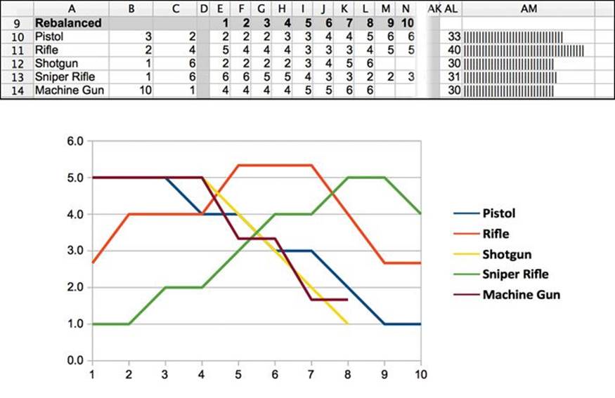
Figure 11.15 The weapon balance chosen for Chapter 9
![]() Even with all this information, some aspects of weapon balance will not be shown in this chart. This includes things like the point made previously about multishot weapons having a much higher chance of dealing the average amount of damage as well as the benefit of the sniper rifle to deal damage to enemies who are too far away to effectively shoot back.
Even with all this information, some aspects of weapon balance will not be shown in this chart. This includes things like the point made previously about multishot weapons having a much higher chance of dealing the average amount of damage as well as the benefit of the sniper rifle to deal damage to enemies who are too far away to effectively shoot back.
Try your hand at balancing the stats for these weapons. You should only change the values in the range B10:N14. Leave the original stats alone, and don’t touch the Percent Chance and Average Damage cells; they will update to reflect the changes you make to the ToHit, Shots, and D/Shot cells. Once you’ve played with this for a while, continue reading.
The Balance Chosen for Chapter 9
In Figure 11.15, you can see the weapon stats that I chose for the prototype in Chapter 9. This is absolutely not the only way to balance these weapons or even the best way to balance them, but it does achieve many of the design goals.
![]() The weapons each have a personality of their own, and none is too overpowered or underpowered.
The weapons each have a personality of their own, and none is too overpowered or underpowered.
![]() Though the shotgun may look a little too similar to the machine gun in its chart, the two guns will feel very different due to two factors: 1. a hit with the 6-damage shotgun is an instant knockout, and 2. the machine Gun fires many bullets, so it will deal average damage much more often.
Though the shotgun may look a little too similar to the machine gun in its chart, the two guns will feel very different due to two factors: 1. a hit with the 6-damage shotgun is an instant knockout, and 2. the machine Gun fires many bullets, so it will deal average damage much more often.
![]() The pistol is pretty decent at close range and is more versatile than the shotgun or machine gun with its ability to attempt to hit enemies at longer range.
The pistol is pretty decent at close range and is more versatile than the shotgun or machine gun with its ability to attempt to hit enemies at longer range.
![]() The rifle really shines at mid-range.
The rifle really shines at mid-range.
![]() The sniper rifle is terrible at close range, but it dominates long distance. A hit with the sniper rifle is 6 points of damage like the shotgun, so it will also take down an enemy in one shot.
The sniper rifle is terrible at close range, but it dominates long distance. A hit with the sniper rifle is 6 points of damage like the shotgun, so it will also take down an enemy in one shot.
Even though this kind of spreadsheet-based balancing doesn’t cover all possible implications of the design of the weapons, it’s still a critical tool to have in your game design arsenal because it can help you understand large amounts of data quickly. Several designers of free-to-play games spend most of their day modifying spreadsheets to make slight tweaks in game balance, so if you’re interested in a job in that field, spreadsheets and data-driven design (like you just did) are very important skills.
Summary
There was a lot of math in this chapter, but I hope you saw that learning a little about math can be very useful for you as a game designer. Most of the topics covered in this chapter could merit their own book or course, so I encourage you to look into them further if your interest has been piqued.
In the next chapter, you learn about the specific discipline of puzzle design. Though games and puzzles are similar, there are some key differences that make puzzle design worth separate consideration.