Discovering Modern C++. An Intensive Course for Scientists, Engineers, and Programmers(2016)

Chapter 7. Scientific Projects

In the preceding chapters, we focused primarily on language features of C++ and how we can best apply them to relatively small study examples. This last chapter should give you some ideas for how to build up larger projects. The first section (§7.1) from the author’s friend Mario Mulansky deals with the topic of interoperability between libraries. It will give you a look behind the curtain at odeint: a generic library that seamlessly inter-operates with several other libraries in a very tight fashion. Then we will provide some background on how executables are built from many program sources and library archives (§7.2.1) and how tools can support this process (§7.2.2). Finally, we discuss how program sources are appropriately distributed over multiple files (§7.2.3).

7.1 Implementation of ODE Solvers

Written by Mario Mulansky

In this section we will go through the major steps for designing a numerical library. The focus here is not to provide the most complete numerical functionality, but rather to arrive at a robust design that ensures maximal generality. As an example, we will consider the numerical algorithms for finding the solution of Ordinary Differential Equations (ODEs). In the spirit of Chapter 3, our aim is to make the implementation as versatile as possible by using generic programming. We start by briefly introducing the mathematical background of the algorithms followed by a simple, straightforward implementation. From this, we will be able to identify individual parts of the implementation and one by one make them exchangeable to arrive at a fully generic library. We are convinced that after studying this detailed example of a generic library design, the reader will be able to apply this technique to other numerical algorithms as well.

7.1.1 Ordinary Differential Equations

Ordinary differential equations are a fundamental mathematical tool to model physical, biological, chemical, or social processes and are one of the most important concepts in science and engineering. Except for a few simple cases, the solution of an ODE cannot be found with analytical methods, and we have to rely on numerical algorithms to obtain at least an approximate solution. In this chapter, we will develop a generic implementation of the Runge-Kutta-4 algorithm, a general-purpose ODE solver widely used due to its simplicity and robustness.

Generally, an ordinary differential equation is an equation containing a function x(t) of an independent variable t and its derivatives x′, x″, . . .:

This is the most general form, including implicit ODEs. However, here we will only consider explicit ODEs, which are of the form x⁽ⁿ⁾ = f(x, x′, x″,. . ., x⁽ⁿ^–1)) and are much simpler to address numerically. The highest derivative n that appears in the ODE is called the order of the ODE. But any ODE of order n can be easily transformed into an n-dimensional ODE of the first order [23]. Therefore, it is sufficient to consider only first-order differential equations where n = 1. The numerical routines presented later will all deal with initial value problems (IVPs): ODEs with a value for xat a starting point x(t = t₀) = x₀. Thus, the mathematical formulation of the problem that will be numerically addressed throughout the following pages is

Here, we use the vector notation to indicate that the variable might be a more-dimensional vector. Typically, the ODE is defined for real-valued variables, i.e., , but it is also possible to consider complex-valued ODEs where . The function is called the right-hand side (RHS) of the ODE. The most simple physical example for an ODE is probably the Harmonic Oscillator, i.e., a point mass connected to a spring. Newton’s equation of motion for such a system is

where q(t) denotes the position of the mass and ω₀ is the oscillation frequency. The latter is a function of the mass m and the stiffness of the spring k: . This can be brought into form (7.2) by introducing p = dq/dt, using and defining some initial conditions, e.g., q(0) = q₀, p(0) = 0. Using the shorthand notation and omitting explicit time dependencies, we get

Note that in Eq. (7.4) does not depend on the variable t, which makes Eq. (7.4) an Autonomous ODE. Also note that in this example the independent variable t denotes the time and a point in phase spaces, hence the solution is the Trajectory of the harmonic oscillator. This is a typical situation in physical ODEs and the reason for our choice of variables t and .¹

1. In mathematics, the independent variable is often called x and the solution is y(x).

For the harmonic oscillator in Eq. (7.4), we can find an analytic solution of the IVP: q(t) = q₀ cos ω₀t and p(t) = –q₀ω₀ sin(ω₀t). More complicated, non-linear ODEs are often impossible to solve analytically, and we have to employ numerical methods to find an approximate solution. One specific family of examples is systems exhibiting Chaotic Dynamics [34], where the trajectories cannot be described in terms of analytical functions. One of the first models where this has been explored is the so-called Lorenz system, a three-dimensional ODE given by the following equations for :

where σ, R, are parameters of the system. Figure 7–1 depicts a trajectory of this system for the typical choice of parameters σ = 10, R = 28, and b = 10/3. For these parameter values the Lorenz system exhibits a so-called Chaotic Attractor, which can be recognized in Figure 7–1.

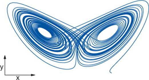
Figure 7–1: Chaotic trajectory in the Lorenz system with parameters σ = 10, R = 28, and b = 10/3

Although such a solution is impossible to find analytically, there are mathematical proofs regarding its existence and uniqueness under some conditions on the RHS , e.g., the Picard-Lindelöf theorem, which requires to be Lipschitz-continuous [48]. Provided that this condition is fulfilled and a unique solution exists—as is the case for almost all practical problems—we can apply an algorithmic routine to find a numerical approximation of this solution.

7.1.2 Runge-Kutta Algorithms

The most common general-purpose schemes for solving initial value problems of ordinary differential equations are the so-called Runge-Kutta (RK) methods [23]. We will focus on the explicit RK schemes as those are easier to implement and well suited for GPUs. They are a family of iterative one-step methods that rely on a temporal discretization to compute an approximate solution of the IVP. Temporal discretization means that the approximate solution is evaluated at time points t_n. So we use for the numerical approximation of the solution x(t_n) at time t_n. In the simplest but most frequently used case of an equidistant discretization with a constant step size Δt, one writes for the numerical solution:

The approximate points are obtained sequentially using a numerical algorithm that can be written in its most general form as

The mapping here represents the numerical algorithm, i.e., the Runge-Kutta scheme, that performs one iteration from to with the time step Δt. The numerical scheme is said to have the order m if the solution it generates is exact up to some error of order m + 1:

where is the exact solution of the ODE at t₁ starting from the initial condition . Hence, m denotes the order of accuracy of a single step of the scheme.

The most basic numerical algorithm to compute such a discrete trajectory x₁, x₂, . . . is the Euler Scheme, where , which means the next approximation is obtained from the current one by

This scheme has no practical relevance because it only offers accuracy of order m = 1. A higher order can be reached by introducing intermediate points and thus dividing one step into several stages. For example, the famous RK4 scheme, sometimes called the Runge-Kutta method, has s = 4 stages and also order m = 4. It is defined as follows:

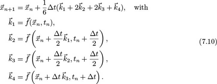
Note how the subsequent computations of the intermediate results depend on the result of the previous stage .

More generally, a Runge-Kutta scheme is defined by its number of stages s and a set of parameters c₁ . . . c_s, a₂₁, a₃₁, a₃₂, . . ., a_ss_–1, and b₁ . . . b_s. The algorithm to calculate the next approximation x_n₊₁ is then given by

The parameter sets a_i,j, b_i, and c_i define the so-called Butcher tableau (see Figure 7–2) and fully describe the specific Runge-Kutta scheme. The Butcher tableau for the RK4 scheme above is given in Figure 7–2(b).

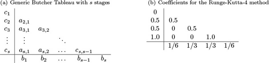
Figure 7–2: Butcher tableaus

7.1.3 Generic Implementation

Implementing the Runge-Kutta scheme introduced above in C++ in a straightforward manner does not create any difficulty. For example, we can use std::vector<double> to represent the state and the derivatives and use a template parameter to allow some generality for the RHS function . The code in Listing 7–1 shows a quick and easy implementation of the Euler scheme introduced above. For simplicity, we restrict our examples to the Euler scheme to keep the code snippets brief, but the following points hold for similar implementations of more complicated Runge-Kutta schemes as well.

Listing 7–1: Basic implementation of the Euler scheme

typedef std::vector<double> state_type;

template<class System>
void euler_step(System system, state_type &x,
const double t, const double dt)
{
state_type k(x.size());
system(x, k, t);
for(int i=0; i<x.size(), ++i)
x[i] += dt*k[i];
}

Defining the RHS system as a template parameter already gives us some nice generality: the euler_step function takes function pointers, as well as functors and C++ lambda objects, as system parameters. The only requirement is that the system object is callable with the parameter structure system(x, dxdt, t) and that it computes the derivative in dxdt.

Although this implementation works perfectly fine in many cases, it has several serious problems as soon as you come across some non-standard situations. Such situations might be

• Different state types, i.e., a fixed-size array (std::array) that might give better performance;

• ODEs for complex numbers;

• Non-standard containers, i.e., for ODEs on complex networks;

• Necessity of higher precision than double;

• Parallelization, e.g., via OpenMP or MPI; and

• Usage of GPGPU devices.

In the following, we will generalize the implementation in Listing 7–1 in such a way that we can deal with the situations mentioned above. Therefore, we will first identify the computational requirements of the Runge-Kutta schemes and then address each of these requirements individually. The result will be a highly modularized implementation of those algorithms that will allow us to exchange specific parts of the computation so that we can provide solutions to the before-mentioned problems.

7.1.3.1 Computational Requirements

To obtain a generic implementation of the Euler scheme (Listing 7–1), we need to separate the algorithm from the implementation details. For that, we first have to identify the computational requirements that are involved in the Euler scheme. From inspecting Eq. (7.9) or (7.10) together with the basic Euler implementation in Listing 7–1, we can identify several required parts for the computation.

First, the mathematical entities have to be represented in the code, namely, the state variable of the ODE as well as the independent variable t and the constants of the Runge-Kutta scheme a, b, c. In Listing 7–1, we use std::vector<double> and double respectively, but in a generic implementation this will become a template parameter. Second, memory allocation has to be performed to store the intermediate results . Furthermore, an iteration over the possibly high-dimensional state variable is required, and finally scalar computation involving the elements of the state variable x_i, the independent variable t, Δt, as well as the numerical constants a, b, c has to be performed. To summarize, the Runge-Kutta schemes introduced before require the following computational components:

1. Representation of mathematical entities,

2. Memory management,

3. Iteration, and

4. Elementary computation.

Having identified those requirements, we can now design a generic implementation where each requirement is addressed by a modularized piece of code that will be exchangeable.

7.1.3.2 Modularized Algorithm

In our modularized design, we will introduce separate code structures for the four requirements identified before. We start with the types used to represent the mathematical objects: the state , the independent variable (time) t, and the parameters of the algorithms a, b, c (Figure 7–2(a)). The standard way to generalize algorithms for arbitrary types is to introduce template parameters. We also follow this approach and hence define three template parameters: state_type, time_type, and value_type. Listing 7–2 shows the class definition of the Runge-Kutta-4 scheme with those template arguments. Note how we use double as the default arguments for value_type and time_type so in most cases only the state_type needs to be specified by the user.

Listing 7–2: Runge-Kutta class with templated types

template<
class state_type,
class value_type = double,
class time_type = value_type
>
class runge_kutta4 {
// ...
};
typedef runge_kutta4< std::vector<double> > rk_stepper;

Next, we address the memory allocation. In Listing 7–1 this is done in terms of the std::vector constructor which expects the vector size as a parameter. With generic state_types, this is not acceptable anymore, as the user might provide other types such as std::array that are not constructed with the same signature. Therefore, we introduce a templated helper function resize that will take care of the memory allocations. This templated helper function can be specialized by the user for any given state_type. Listing 7–3 shows the implementation forstd::vector and std::array as well as its usage in the runge_kutta4 implementation. Note how the resize function allocates memory for the state out based on the state in. This is the most general way to implement such memory allocation; it also works for sparse matrix types where the required size is not so trivial. The resizing approach in Listing 7–3 provides the same functionality as the non-generic version in Listing 7–1 as again the runge_kutta4 class is responsible for its own memory management. It immediately works with any vector type that provides resize and size functions. For other types, the user can provide resize overloads and in that way tell the runge_kutta4 class how to allocate memory.

Next are the function calls to compute the RHS equation . This is already implemented in a generic way in Listing 7–1 by means of templates, and we will keep this solution.

Finally, we have to find abstractions for the numerical computations. As noted above, this involves iteration over the elements of and the basic computations (summation, multiplication) on those elements. We address both parts separately by introducing two code structures: Algebraand Operation. While Algebra will handle the iterations, Operation will be in charge of the computations.

We start with Algebra. For the RK4 algorithm, we need two functions that iterate over three and six instances of state_type respectively. Keeping in mind that the state_type typically is a std::vector or std::array, it is reasonable to provide an algebra that can deal with C++ containers. To ensure as much generality as possible for our basic algebra, we will use the std::begin and std::end functions introduced with C++11 as part of the standard library.

Listing 7–3: Memory allocation

template<class state_type>
void resize(const state_type &in, state_type &out) {
// standard implementation works for containers
using std::size;
out.resize(size(in));
}

// specialization for std::array
template<class T, std::size_t N>
void resize(const std::array<T, N> &, std::array<T,N>& ) {
/* arrays don't need resizing */
}

template< ... >
class runge_kutta4 {
// ...
template<class Sys>
void do_step(Sys sys, state_type &x,
time_type t, time_type dt)
{
adjust_size(x);
// ...
}

void adjust_size(const state_type &x) {
resize(x, x_tmp);
resize(x, k1);
resize(x, k2);
resize(x, k3);
resize(x, k4);
}
};

Advice

The correct way to use free functions such as std::begin in a generic library is by locally lifting them into the current namespace with using std::begin and then accessing them without a namespace qualifier, i.e., begin(x), as is done in Listing 7–4. This way, the compiler can also utilize begin functions defined in the same namespace as the type of x via argument-dependent name lookup (ADL) if necessary.

Listing 7–4 shows such a container_algebra. The iterations are performed within for_each functions that are part of the struct called container_algebra. Those functions expect a number of container objects as well as an operation object and then simply perform an iteration over all containers and execute the given operation element-wise. The Operation performed for each element is a simple multiplication and addition and will be described next.

Listing 7–4: Container algebra

struct container_algebra
{
template<class S1, class S2, class S3, class Op>
void for_each3(S1 &s1, S2 &s2, S3 &s3, Op op) const
{
using std::begin;
using std::end;

auto first1 = begin(s1);
auto last1 = end(s1);
auto first2 = begin(s2);
auto first3 = begin(s3);
for( ; first1 != last1 ; )
op(*first1++, *first2++, *first3++);
}
};

The final pieces are the fundamental operations that will consist of functor objects again gathered in a struct. Listing 7–5 shows the implementation of those operation functors. For simplicity, we again present only the scale_sum2 functor that can be used in for_each3 (Listing 7–4). However, the extension to scale_sum5 to work with for_each6 is rather straightforward. As seen in Listing 7–5, the functors consist of a number of parameters alpha1, alpha2,.. and a function call operator that computes the required product-sum.

Listing 7–5: Operations

struct default_operations {
template<class F1=double, class F2=F1>
struct scale_sum2 {
typedef void result_type;

const F1 alpha1;
const F2 alpha2;

scale_sum2(F1 a1, F2 a2)
: alpha1(a1), alpha2(a2) { }

template<class T0, class T1, class T2>
void operator()(T0 &t0, const T1 &t1, const T2 &t2) const
{
t0 = alpha1 * t1 + alpha2 * t2;
}
};
};

Having collected all the modularized ingredients, we can implement the Runge-Kutta-4 algorithm based on the parts described above. Listing 7–6 shows this implementation. Note how all the parts introduced above are supplied as template parameters and are therefore configurable.

Listing 7–6: Generic Runge-Kutta-4

template<class state_type, class value_type = double,
class time_type = value_type,
class algebra = container_algebra,
class operations = default_operations>
class runge_kutta4 {
public:
template<typename System>
void do_step(System &system, state_type &x,
time_type t, time_type dt)
{
adjust_size( x );
const value_type one = 1;
const time_type dt2 = dt/2, dt3 = dt/3, dt6 = dt/6;

typedef typename operations::template scale_sum2<
value_type, time_type> scale_sum2;

typedef typename operations::template scale_sum5<
value_type, time_type, time_type,
time_type, time_type> scale_sum5;

system(x, k1, t);
m_algebra.for_each3(x_tmp, x, k1, scale_sum2(one, dt2));

system(x_tmp, k2, t + dt2);
m_algebra.for_each3(x_tmp, x, k2, scale_sum2(one, dt2));

system(x_tmp, k3, t + dt2);
m_algebra.for_each3(x_tmp, x, k3, scale_sum2(one, dt));

system(x_tmp, k4, t + dt);
m_algebra.for_each6(x, x, k1, k2, k3, k4,
scale_sum5(one, dt6, dt3,
dt3, dt6));
}
private:
state_type x_tmp, k1, k2, k3, k4;
algebra m_algebra;

void adjust_size(const state_type &x) {
resize(x, x_tmp);
resize(x, k1); resize(x, k2);
resize(x, k3); resize(x, k4);
}
};

The following code snippet shows how this Runge-Kutta-4 stepper can be instantiated:

typedef runge_kutta4< vector<double>, double, double ,
container_algebra,
default_operations> rk4_type;
// equivalent shorthand definition using the default parameters:
// typedef runge_kutta4< vector<double> > rk4_type;

rk_stype rk4;

7.1.3.3 A Simple Example

In the end, we present a small example of how to use the generic Runge-Kutta-4 implementation above to integrate a trajectory of the famous Lorenz system. Therefore, we only have to define the state type, implement the RHS equation of the Lorenz system, and then use therunge_kutta4 class from above with the standard container_algebra and default_operations. Listing 7–7 shows an example implementation requiring only 30 lines of C++ code.

7.1.4 Outlook

We have arrived at a generic implementation of the Runge-Kutta-4 scheme. From here, we can continue in numerous directions. Obviously, more Runge-Kutta schemes can be added, potentially including step-size control and/or dense output facility. Although such methods might be more difficult to implement and will require more functionality from the back ends (algebra and operations), they conceptually fit into the generic framework outlined above. Also, it is possible to expand to other explicit algorithms such as multi-step methods or predictor-corrector schemes, as essentially all explicit schemes only rely on RHS evaluations and vector operations as presented here. Implicit schemes, however, require higher-order algebraic routines like solving linear systems and therefore would need a different class of algebra than the one introduced here.

Furthermore, we can provide other back ends besides container_algebra. One example could be to introduce parallelism with omp_algebra or mpi_algebra. Also, GPU computing could be addressed, e.g., by opencl_algebra and the corresponding data structures. Another use case would be to rely on some linear-algebra package that provides vector or matrix types which already implement the required operations. There, no iteration is required and a dummy algebra should be used that simply forwards the desired computation to thedefault_operations without iterating.

As you can see, the generic implementation offers ample ways to adjust the algorithm to non-standard situations, like different data structures or GPU computing. The strength of this approach is that the actual algorithm does not need to be changed. The generality allows us to replace certain parts of the implementation to adapt to different circumstances, but the implementation of the algorithm remains.

An expansive realization of generic ODE algorithms following the approach described here is found in the Boost.odeint library.² It includes numerous numerical algorithms and several back ends, e.g., for parallelism and GPU computing. It is actively maintained and widely used and tested. Whenever possible, it is strongly recommended to use this library instead of reimplementing these algorithms. Otherwise, the ideas and code presented above could serve as a good starting point to implement new, more problem-specific routines in a generic way.

2. http://www.odeint.com

Listing 7–7: Trajectory in the Lorenz system

typedef std::vector<double> state_type;
typedef runge_kutta4< state_type > rk4_type;

struct lorenz {
const double sigma, R, b;
lorenz(const double sigma, const double R, const double b)
: sigma(sigma), R(R), b(b) { }

void operator()(const state_type &x, state_type &dxdt,
double t)
{
dxdt[0] = sigma * ( x[1] - x[0] );
dxdt[1] = R * x[0] - x[1] - x[0] * x[2];
dxdt[2] = -b * x[2] + x[0] * x[1];
}
};

int main() {
const int steps = 5000;
const double dt = 0.01;

rk4_type stepper;
lorenz system(10.0, 28.0, 8.0/3.0);
state_type x(3, 1.0);
x[0] = 10.0; // some initial condition
for( size_t n=0 ; n<steps ; ++n ) {
stepper.do_step(system, x, n*dt, dt);
std::cout n*dt ' ';
std::cout x[0] ' ' x[1] ' ' x[2]
std::endl;
}
}

7.2 Creating Projects

How we design our programs is not really critical as long as they are short. For larger software projects, of say over 100,000 lines of code, it is vital that the sources are well structured. First of all, the program sources must be distributed in a well-defined manner over files. How large or small single files should be varies from project to project and is out of this book’s scope. Here, we only demonstrate basic principles.

7.2.1 Build Process

The build process from source files to executables contains four steps. Nonetheless, many programs with few files can be built with a single compiler call. Thus, the term “compilation” is used ambiguously for the actual compilation step (§7.2.1.2) and the entire build process when performed by a single command.

Figure 7–3 depicts the four steps: preprocessing, compilation, assembly, and linkage. The following sections will discuss these steps individually.

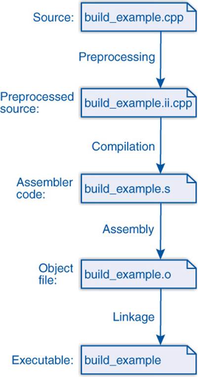
Figure 7–3: Simple build

7.2.1.1 Preprocessing

c++03/build_example.cpp

The (direct) input of the preprocessing is a source file containing implementations of functions and classes. For a C++ project, this is a file with one of the following typical extensions: .cpp, .cxx, .C, .cc, or .c++,³ for instance, build_example.cpp:

3. File name extensions are just conventions and do not matter to the compiler. We could use .bambi as an extension for our programs and they would still compile. The same applies to all other extensions in the remainder of this build discussion.

#include <iostream>
#include <cmath>

int main (int argc, char* argv[])
{
std::cout "sqrt(17) is " sqrt(17) '\n';
}

c++03/build_example.ii.cpp

The indirect inputs are all files included by the corresponding #include directive. These includes are header files containing declarations. The inclusion is a recursive process that expands to the includes of the includes and so on. The result is a single file containing all direct and indirect include files. Such an expanded file can consist of several hundred thousand lines when large third-party libraries with massive dependencies like Boost are included. Only including <iostream> inflates small programs like the preceding toy example to about 20,000 lines:

# 1 "build_example.cpp"
# 1 "<command-line>"
// ... skipped some lines here
# 1 "/usr/include/c++/4.8/iostream" 1 3
# 36 "/usr/include/c++/4.8/iostream" 3
// ... skipped some lines here
# 184 "/usr/include/x86_64-linux-gnu/c++/4.8/bits/c++config.h" 3
namespace std
{
typedef long unsigned int size_t;
// ... skipped many, many lines here
# 3 "build_example.cpp" 2

int main (int argc, char* argv[])
{
std::cout "sqrt(17) is " sqrt(17) '\n';
}

Preprocessed C++ programs usually get the extension .ii (.i for preprocessed C). To execute the preprocessing only, use the compiler flag -E (/E for Visual Studio). The output should be specified with -o; otherwise it is printed on the screen.

In addition to the inclusion, macros are expanded and conditional code selected. The whole preprocessing step is pure text substitution, mostly independent (ignorant) of the programming language. As a consequence, it is very flexible but also extremely error-prone as we discussed inSection 1.9.2.1. The set of files that are merged during the preprocessing is called a Translation Unit.

7.2.1.2 Compilation

c++03/build_example.s

The (actual) compilation translates the preprocessed sources into assembler code of the target platform.⁴ This is a symbolic representation of the platform’s machine language, e.g.:

4. A C++ compiler is not obliged by the standard to generate assembler code but all common compilers do so.

.file "build_example.cpp"
.local _ZStL8__ioinit
.comm _ZStL8__ioinit,1,1
.section .rodata
.LC0:
.string "sqrt(17) is "
.text
.globl main
.type main, @function
main:
.LFB1055:
.cfi_startproc
pushq %rbp
.cfi_def_cfa_offset 16
.cfi_offset 6, -16
movq %rsp, %rbp
.cfi_def_cfa_register 6
subq $32, %rsp
movl %edi, -4(%rbp)
movq %rsi, -16(%rbp)
movl $.LC0, %esi
movl $_ZSt4cout, %edi
call _ZStlsISt11char_traitsIcEERSt13basic_ostreamIcT_ES5_PKc
movq %rax, %rdx
; just a bit more code

Surprisingly, the assembler code is much shorter (92 lines) than the preprocessed C++ for this example because it only contains the operations that are really performed. Typical extensions for assembler programs are .s and .asm.

The compilation is the most sophisticated part of the build process where all the language rules of C++ apply. The compilation itself consists of multiple phases: front end, middle end, and back end, which in turn can consist of multiple passes.

In addition to the code generation, the names of the C++ program are decorated with type and namespace (§3.2.1) information. This decoration is called Name Mangling.

7.2.1.3 Assembly

The assembly is a simple one-to-one transformation from the assembler into the machine language where the commands are replaced by hexadecimal code and labels by true (relative) addresses. The resulting files are called Object Code and their extension is usually .o and on Windows.obj. The entities in the object files (code snippets and variables) are called Symbols.

Object files can be bundled to archives (extensions .a, .so, .lib, .dll, and the like). This process is entirely transparent to the C++ programmer and there is nothing that we can do wrong such that we get errors in this part of the build process.

7.2.1.4 Linking

In the last step, the object files and archives are Linked together. The two main tasks of the linker are

• Matching the symbols of different object files, and

• Mapping addresses relative to each object file onto the application’s address space.

In principle, the linker has no notion of types and matches the symbols only by name. Since, however, the names are decorated with type information, a certain degree of type safety is still provided during linkage. The name mangling allows for linking function calls with the right implementation when the function is overloaded.

Archives—also called link libraries—are linked in two fashions:

• Statically: The archive is entirely contained in the executable. This linkage is applied to .a libraries on Unix systems and .lib libraries on Windows.

• Dynamically: The linker only checks the presence of all symbols and keeps some sort of reference to the archive. This is used for .so (Unix) and .dll (Windows) libraries.

The impact is obvious: executables that are linked against dynamic libraries are much smaller but depend on the presence of the libraries on the machine where the binary is executed. When a dynamic library is not found on Unix/Linux, we can add its directory to the search path in the environment LD_LIBRARY_PATH. On Windows, it requires a little more work.

7.2.1.5 The Complete Build

Figure 7–4 illustrates how the application for a flux simulator might be generated. First we preprocess the main application in fluxer.cpp which includes standard libraries like <iostream> and domain-specific libraries for meshing and solving. The expanded source is then compiled to the object file fluxer.o. Finally, the application’s object file is linked with standard libraries like libstdc++.so and the domain libraries whose headers we included before. Those libraries can be linked statically like libsolver.a or dynamically like libmesher.so. Frequently used libraries like those from the system are often available in both forms.

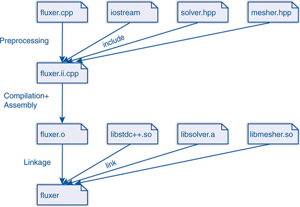
Figure 7–4: Complex build

7.2.2 Build Tools

When we build our applications and libraries from program sources and already-compiled libraries, we can either type in lots of commands over and over or use suitable tools. In this section, we present two of the latter: make and CMake. As a case study we consider a scenario like in Figure 7–4: a fluxer application that is linked with a mesher and a solver library which in turn are built from the appropriate source and header files.

7.2.2.1 make

buildtools/makefile

We do not know what you have heard about make, but it is not as bad as its reputation.⁵ Actually it works pretty well for small projects. The basic idea is that we express dependencies between targets and their sources, and when a target is older than its sources or missing, that target is generated with the given commands. These dependencies are written to a makefile and automatically resolved by make. In our example, we have to compile fluxer.cpp to the corresponding object file fluxer.o:

5. Rumor has it that its author showed it to his colleagues before leaving on vacation. When he came back, already regretting the design, it was being used all over the company and it was too late to retract it.

fluxer.o: fluxer.cpp mesher.hpp solver.hpp
g++ fluxer.cpp -c -o fluxer.o

The line(s) with the command(s) must start with a tabulator. As the rules for all object files are similar enough, we write a generic rule instead for all that originate from C++ sources:

.cpp.o:
${CXX} ${CXXFLAGS} $^ -c -o $@

The variable ${CXX} is preset to the default C++ compiler and ${CXXFLAGS} to its default flags. We can change these variables:

CXX= g++-5
CXXFLAGS= -O3 -DNDEBUG # Release
# CXXFLAGS= -O0 -g # Debug

Here we changed the compiler or applied aggressive optimization (for release mode). As a comment, we also demonstrated the debug mode with no optimization and symbol tables within object files needed by debugging tools. We used automatic variables: $@ for the rule’s target and $^ for its sources. Next we have to build our mesher and solver libraries:

libmesher.a: mesher.o # more mesher sources
ar cr $@ $^

libsolver.a: solver.o # more solver sources
ar cr $@ $^

For simplicity we build both with static linkage (deviating from Figure 7–4). Finally, we link the application and the libraries together:

fluxer: fluxer.o libmesher.a libsolver.a
${CXX} ${CXXFLAGS} $^ -o $@

If we used the default linker instead of the C++ compiler here, we would need to add C++ standard libraries and possibly some flags specific to C++ linkage. Now we can build our project with one single command:

make fluxer

This triggers the following commands:

g++ fluxer.cpp -c -o fluxer.o
g++ mesher.cpp -c -o mesher.o
ar cr libmesher.a mesher.o
g++ solver.cpp -c -o solver.o
ar cr libsolver.a solver.o
g++ fluxer.o libmesher.a libsolver.a -o fluxer

If we change mesher.cpp, the next build process only generates targets depending on it:

g++ mesher.cpp -c -o mesher.o
ar cr libmesher.a mesher.o
g++ fluxer.o libmesher.a libsolver.a -o fluxer

By convention, the first target not starting with a dot is considered the default target:

all: fluxer

so we can just write make.

7.2.2.2 CMake

buildtools/CMakeLists.txt

CMake is a tool of higher abstraction than make as we will demonstrate in this section. Our build project is specified here in a file named CMakeLists.txt. It typically starts with declaring which tool version is needed and naming a project:

cmake_minimum_required (VERSION 2.6)
project (Fluxer)

Generating a new library is easily done by just declaring its sources:

add_library(solver solver.cpp)

Which commands are used and how they are parameterized is decided by CMake unless we insist on more detailed specification. A library with dynamic linkage can be generated as easily:

add_library(mesher SHARED mesher.cpp)

Our final goal is the creation of the fluxer application that is linked against these two libraries:

add_executable(fluxer fluxer.cpp)
target_link_libraries(fluxer solver mesher)

It is good practice to build CMake projects in separate directories so that we can toss all generated files at once. One typically creates a sub-directory named build and runs all commands there:

cd build
cmake ..

Now CMake searches for compilers and other tools, including their flags:

-- The C compiler identification is GNU 4.9.2
-- The CXX compiler identification is GNU 4.9.2
-- Check for working C compiler: /usr/bin/cc
-- Check for working C compiler: /usr/bin/cc -- works
-- Detecting C compiler ABI info
-- Detecting C compiler ABI info - done
-- Check for working CXX compiler: /usr/bin/c++
-- Check for working CXX compiler: /usr/bin/c++ -- works
-- Detecting CXX compiler ABI info
-- Detecting CXX compiler ABI info - done
-- Configuring done
-- Generating done
-- Build files have been written to: ... /buildtools/build

Finally it builds a makefile that we call now:

make

Running:

Scanning dependencies of target solver
[ 33%] Building CXX object CMakeFiles/solver.dir/solver.cpp.o
Linking CXX static library libsolver.a
[ 33%] Built target solver
Scanning dependencies of target mesher
[ 66%] Building CXX object CMakeFiles/mesher.dir/mesher.cpp.o
Linking CXX shared library libmesher.so
[ 66%] Built target mesher
Scanning dependencies of target fluxer
[100%] Building CXX object CMakeFiles/fluxer.dir/fluxer.cpp.o
Linking CXX executable fluxer
[100%] Built target fluxer

The generated makefiles reflect the dependencies, and when we change some sources the next make will only rebuild what is affected by the changes. In contrast to our simplistic makefile from Section 7.2.2.1, modified header files are considered here. If we changed, for instance,solver.hpp, libsolver.a and fluxer would be freshly built.

The biggest benefit we kept for the end: CMake’s portability. From the same CMakeLists.txt file from which we generated makefiles, we can create a Visual Studio project by just using another generator. The author enjoyed this feature a lot: till today he never created a Visual Studio project himself but generated them all with CMake. Nor did he migrate these projects to newer Visual Studio versions. Instead he just created new projects with new versions of the generators. Likewise one can generate Eclipse and XCode projects. KDevelop can build its projects fromCMake files and even update them. In short, it is a really powerful build tool and at the time of writing probably the best choice for many projects.

7.2.3 Separate Compilation

Having seen how we can build an executable from multiple sources, we will now discuss how those sources should be designed for avoiding conflicts.

7.2.3.1 Headers and Source Files

Each unit of source code is typically split into

• A header file with declarations (e.g., .hpp), and

• A source file (e.g., .cpp).

The source file contains the realization of all algorithms from which the executable will be generated.⁶ The header file contains declarations of the functions and classes that are implemented in the other file. Some functions may be used only internally and thus omitted in the header file. For instance, the math functions of our friend Herbert will be split into

6. The terminology is not mathematically sharp: inline and template functions are defined in headers.

// File: herberts/math_functions.hpp
#ifndef HERBERTS_MATH_FUNCTIONS_INCLUDE
#define HERBERTS_MATH_FUNCTIONS_INCLUDE

typedef double hreal; // Herbert's real numbers

hreal sine(hreal);
hreal cosine(hreal);
...
# endif

// File: herberts/math_functions.cpp
#include <herberts/math_functions.hpp>

hreal divide_by_square(hreal x, hreal y) { ... }

hreal sine(hreal) { ... }
hreal cosine(hreal) { ... }
...

We leave it to the reader’s fantasy why Herbert introduced his own real number type.

To use Herbert’s magnificent functions, we need two things:

• The declarations by

– Including the header file herberts/math_functions.hpp or

– Declaring all desired functions ourselves.

• The compiled code by

– Linking against math_functions.o (.obj under Windows) or

– Linking against a library containing math_functions.o.

The declarations tell the compiler that the code for the functions with the given signatures exists somewhere and that they can be called in the current compilation unit.

The linkage step then brings together the function calls with their actual code. The simplest way to link the compiled functions to some application is passing the object file or the archive as an argument to the C++ compiler. Alternatively, we could use a standard linker, but then we would need a handful of C++-specific extra flags.

7.2.3.2 Linkage Problems

During the linkage, the C++ entities like functions and variables are represented by symbols. C++ uses Name Mangling: decorating the symbol names with type and namespace (§3.2.1) information.

There are three things that can go wrong during the linkage:

1. Symbols (functions or variables) are not found;

2. Symbols are found twice; or

3. There is no main function (or multiple).

Not finding a symbol can have different causes:

• The symbols for the declaration and the implementation do not match.

• The corresponding object file or archive is not linked.

• The archives are linked in the wrong order.

A missing symbol is in most cases just a typo. As the symbol names contain type information due to name mangling, it can also be a type mismatch. Another possibility is that the source code is compiled with incompatible compilers where the names are mangled differently.

To avoid problems during linkage or execution, it must be verified that all sources are compiled with compatible compilers; i.e., names are equally mangled and function arguments placed in the same order on the stack. This does not only apply to our own object files and those of third-party libraries but also to the C++ standard library which is always linked in. In Linux, one should use the default compiler which is guaranteed to work with all precompiled software packages. If an older or newer compiler version is not available as a package, it is often an indicator of compatibility issues. It can still be used, but this is perceivably more work (manual installation, careful configuration of our own build processes, . . . ).

When the linker complains about redefinition of symbols, it is possible that the same name is declared and used in multiple implementations. More often it is caused by defining variables and functions in header files. This works as long as such a header is only included in one translation unit. When headers with (certain) definitions are included more than once, the linkage fails.

For illustration purposes, we come back to our friend Herbert’s infamous math functions. Next to many magnificent math functions, the header contains the following critical definitions:

// File: herberts/math_functions.hpp
..
double square(double x) { return x*x; }
double pi= 3.14159265358979323846264338327950288419716939;

After including this header into multiple translation units, the linker will complain:

g++-4.8 -o multiref_example multiref1.cpp multiref2.cpp
/tmp/cc65d1qC.o:(.data+0x0): multiple definition of 'pi'
/tmp/cc1slHbY.o:(.data+0x0): first defined here
/tmp/cc65d1qC.o: In function 'square(double)':
multiref2.cpp:(.text+0x0): multiple definition of 'square(double)'
/tmp/cc1slHbY.o:multiref1.cpp:(.text+0x63): first defined here
collect2: error: ld returned 1 exit status

Let us first deal with the function and then with the variable.

The first aid against redefinition is static:

static double square(double x) { return x*x; }

It declares the function local to the translation unit. The C++ standard calls this Internal Linkage (as opposed to external linkage evidently). The drawback is code replication: when the header is included n times, the function’s code appears n times in the executable.

An inline declaration:

inline double square(double x) { return x*x; }

has a similar effect. Whether or not the function is actually inlined, an inline function always has internal linkage.⁷ Conversely, functions without an inline specifier have external linkage and cause linker errors even when the programmer chooses to inline them.

7. Advanced: In contrast to static functions, the code is not necessarily replicated. Instead it can be represented by a weak symbol that causes no linker error in redefinitions.

Alternatively, we can avoid the redefinition by defining the function in only one translation unit:

// File: herberts/math_functions.hpp
double square(double x);

// File: herberts/math_functions.cpp
double square(double x) { return x*x; }

This is the preferable approach for large functions.

Function Definition

Short functions should be inline and defined in headers. Large functions should be declared in headers and defined in source files.

For data, we can use similar techniques. A static variable:

static double pi= 3.14159265358979323846264338327950288419716939;

is replicated in all translation units. This solves our linker problem but probably causes others as the following not-so-smart example illustrates:

// File: multiref.hpp
static double pi= 17.4;

// File: multiref1.cpp
int main (int argc, char* argv[])
{
fix_pi();
std::cout "pi = " pi std::endl;
}

// File: multiref1.cpp
void fix_pi() { pi= 3.14159265358979323846264338327950288419716939; }

It is better to define it once in a source file and declare it in the header using the attribute extern:

// File: herberts/math_functions.hpp
extern double pi;

// File: herberts/math_functions.cpp
double pi= 3.14159265358979323846264338327950288419716939;

Finally, we will do the most reasonable: declaring π as a constant. Constants also have internal linkage⁸ (unless previously declared extern) and can be safely defined in header files:

8. Advanced: They may be stored only once as weak symbols in the executable.

// File: herberts/math_functions.hpp
const double pi= 3.14159265358979323846264338327950288419716939;

Headers should not contain ordinary functions and variables.

7.2.3.3 Linking to C Code

Many scientific libraries are written in C, e.g., PETSc. To use them in C++ software, we have two options:

• Compile the C code with a C++ compiler or

• Link the compiled code.

C++ started as a superset of C. C99 introduced some features that are not part of C++ and even in old C there exist some academic examples that are not legal C++ code. However, in practice most C programs can be compiled with a C++ compiler.

For incompatible C sources or software that is only available in compiled form, it is possible to link the C binaries to C++ applications. However, C has no name mangling like C++. As a consequence, function declarations are mapped to different symbols by C and C++ compilers.

Say our friend Herbert developed in C the best algorithm for cubic roots, ever. Hoping for a Fields medal, he refuses to provide us the sources. As a great scientist he takes the liberty of stubbornness and feels that compiling his secret C functions with a C++ compiler would desecrate them. However, in his infinite generosity, he offers us the compiled code. To link it, we need to declare the functions with C naming (without mangling):

extern "C" double cubic_root(double);
extern "C" double fifth_root(double);
...

To save some typing, we can use the block notation:

extern "C" {
double cubic_root(double);
double fifth_root(double);
...
}

Later he became even more generous and offered us his precious header file. With that we can declare the entire set of functions as C code with a so-called Linkage Block:

extern "C" {
#include <herberts/good_ole_math_functions.h>
}

In this style, <math.h> is included in <cmath>.

7.3 Some Final Words

I hope you have enjoyed reading this book and are eager to apply many of the freshly learned techniques in your own projects. It was not my intention to cover all facets of C++; I tried my best to demonstrate that this powerful language can be used in many different ways and provide both expressiveness and performance. Over time you will find your own personal way of making the best use of C++. “Best use” was a fundamental criterion for me: I did not want to enumerate uncountable features and all subtleties vaguely related to the language but rather to show which features or techniques would best help you reach your goals.

In my own programming, I have spent a lot of time squeezing out as much performance as possible and have conveyed some of that knowledge in this book. Admittedly, such tuning is not always fun, and writing C++ programs without ultimate performance requirements is much easier. And even without playing the nastiest tricks, C++ programs are still in most cases clearly faster than those written in other languages.

Thus, before focusing on performance, pay attention to productivity. The most precious resource in computing is not the processor time or the memory but your development time. And no matter how focused you are, it always takes longer than you think. A good rule of thumb is to make an initial guess, multiply it by two, and then use the next-larger time unit. The additional time is okay if it leads to a program or computing result that really makes a difference. You have my wholehearted wishes for that.