The C++ Programming Language (2013)
Part IV: The Standard Library
40. Numerics
The purpose of computing is insight, not numbers.
– R. W. Hamming
... but for the student,
numbers are often the best road to insight.
– A. Ralston
• Introduction
• Numerical Limits
Limit Macros
• Standard Mathematical Functions
• complex Numbers
• A Numerical Array: valarray
Constructors and Assignments; Subscripting; Operations; Slices; slice_array; Generalized Slices
• Generalized Numerical Algorithms
accumulate(); inner_product(); partial_sum() and adjacent_difference(); iota()
• Random Numbers
Engines; Random Device; Distributions; C-Style Random Numbers
• Advice
40.1. Introduction
C++ was not designed primarily with numeric computation in mind. However, numeric computation typically occurs in the context of other work – such as database access, networking, instrument control, graphics, simulation, and financial analysis – so C++ becomes an attractive vehicle for computations that are part of a larger system. Furthermore, numeric methods have come a long way from being simple loops over vectors of floating-point numbers. Where more complex data structures are needed as part of a computation, C++’s strengths become relevant. The net effect is that C++ is widely used for scientific, engineering, financial, and other computation involving sophisticated numerics. Consequently, facilities and techniques supporting such computation have emerged. This chapter describes the parts of the standard library that support numerics. I make no attempt to teach numeric methods. Numeric computation is a fascinating topic in its own right. To understand it, you need a good course in numerical methods or at least a good textbook – not just a language manual and tutorial.
In addition to the standard-library facilities described here, Chapter 29 is an extended example of numerical programming: an N-dimensional matrix.
40.2. Numerical Limits
To do anything interesting with numbers, we typically need to know something about the general properties of built-in numeric types. To allow the programmer to best take advantage of hardware, these properties are implementation-defined rather than fixed by the rules of the language itself (§6.2.8). For example, what is the largest int? What is the smallest positive float? Is a double rounded or truncated when assigned to a float? How many bits are there in a char?
Answers to such questions are provided by the specializations of the numeric_limits template presented in <limits>. For example:
void f(double d, int i)
{
char classification[numeric_limits<unsigned char>::max()];
if (numeric_limits<unsigned char>::digits==numeric_limits<char>::digits) {
// chars are unsigned
}
if (i<numeric_limits<short>::min() || numeric_limits<short>::max()<i) {
// i cannot be stored in a short without loss of digits
}
if (0<d && d<numeric_limits<double>::epsilon()) d = 0;
if (numeric_limits<Quad>::is_specialized) {
// limits information is available for type Quad
}
}
Each specialization provides the relevant information for its argument type. Thus, the general numeric_limits template is simply a notational handle for a set of constants and constexpr functions:
template<typename T>
class numeric_limits {
public:
static const bool is_specialized = false; // is information available for numeric_limits<T>?
// ... uninteresting defaults ...
};
The real information is in the specializations. Each implementation of the standard library provides a specialization of numeric_limits for each fundamental numeric type (the character types, the integer types, the floating-point types, and bool) but not for any other plausible candidates such as void, enumerations, or library types (such as complex<double>).
For an integral type such as char, only a few pieces of information are of interest. Here is numeric_limits<char> for an implementation in which a char has 8 bits and is signed:
template<>
class numeric_limits<char> {
public:
static const bool is_specialized = true; // yes, we have information
static const int digits = 7; // number of bits ("binary digits") excluding sign
static const bool is_signed = true; // this implementation has char signed
static const bool is_integer = true; // char is an integral type
static constexpr char min() noexcept { return –128; } // smallest value
static constexpr char max() noexcept { return 127; } // largest value
// lots of declarations not relevant to a char
};
The functions are constexpr, so that they can be used where a constant expression is required and without run-time overhead.
Most members of numeric_limits are intended to describe floating-point numbers. For example, this describes one possible implementation of float:
template<>
class numeric_limits<float> {
public:
static const bool is_specialized = true;
static const int radix = 2; // base of exponent (in this case, binary)
static const int digits = 24; // number of radix digits in mantissa
static const int digits10 = 9; // number of base 10 digits in mantissa
static const bool is_signed = true;
static const bool is_integer = false;
static const bool is_exact = false;
static constexpr float min() noexcept { return 1.17549435E–38F; } // smallest positive
static constexpr float max() noexcept { return 3.40282347E+38F; } // largest positive
static constexpr float lowest() noexcept { return –3.40282347E+38F; } // smallest value
static constexpr float epsilon() noexcept { return 1.19209290E–07F; }
static constexpr float round_error() noexcept { return 0.5F; } // maximum rounding error
static constexpr float infinity() noexcept { return /* some value */; }
static constexpr float quiet_NaN() noexcept { return /* some value */; }
static constexpr float signaling_NaN() noexcept { return /* some value */; }
static constexpr float denorm_min() noexcept { return min(); }
static const int min_exponent = –125;
static const int min_exponent10 = –37;
static const int max_exponent = +128;
static const int max_exponent10 = +38;
static const bool has_infinity = true;
static const bool has_quiet_NaN = true;
static const bool has_signaling_NaN = true;
static const float_denorm_style has_denorm = denorm_absent;
static const bool has_denorm_loss = false;
static const bool is_iec559 = true; // conforms to IEC-559
static const bool is_bounded = true;
static const bool is_modulo = false;
static const bool traps = true;
static const bool tinyness_before = true;
static const float_round_style round_style = round_to_nearest;
};
Note that min() is the smallest positive normalized number and that epsilon is the smallest positive floating-point number such that 1+epsilon–1 is larger than 0.
When defining a scalar type along the lines of the built-in ones, it is a good idea also to provide a suitable specialization of numeric_limits. For example, if I write a quadruple-precision type Quad, a user could reasonably expect me to provide numeric_limits<Quad>. Conversely, if I use a nonnumeric type, Dumb_ptr, I would expect for numeric_limits<Dumb_ptr<X>> to be the primary template that has is_specialized set to false, indicating that no information is available.
We can imagine specializations of numeric_limits describing properties of user-defined types that have little to do with floating-point numbers. In such cases, it is usually better to use the general technique for describing properties of a type than to specialize numeric_limits with properties not considered in the standard.
40.2.1. Limit Macros
From C, C++ inherited macros that describe properties of integers. They are found in <climits>:
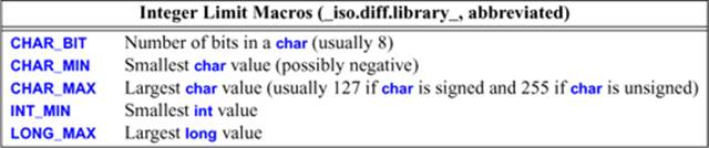
Analogously named macros for signed chars, long long, etc., are also provided.
Similarly, <cfloat> and <float.h> define macros describing properties of floating-point numbers:
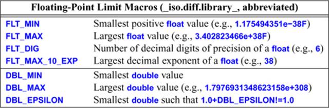
Analogously named macros for long double are also provided.
40.3. Standard Mathematical Functions
In <cmath> we find what are commonly called the standard mathematical functions:
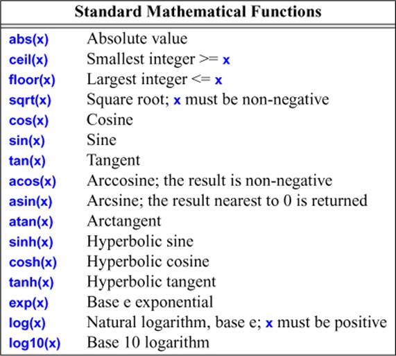
There are versions taking float, double, long double, and complex (§40.4) arguments. For each function, the return type is the same as the argument type.
Errors are reported by setting errno from <cerrno> to EDOM for a domain error and to ERANGE for a range error. For example:
void f()
{
errno = 0; // clear old error state
sqrt(–1);
if (errno==EDOM) cerr << "sqrt() not defined for negative argument";
pow(numeric_limits<double>::max(),2);
if (errno == ERANGE) cerr << "result of pow() too large to represent as a double";
}
For historical reasons, a few mathematical functions are found in <cstdlib> rather than in <cmath>:
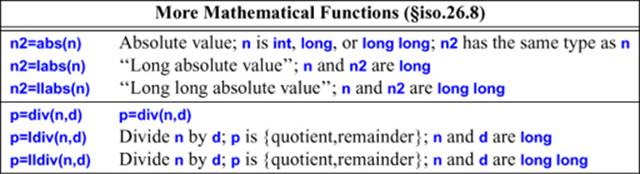
The l*() versions are there because C does not support overloading. The results of the ldiv() functions are structs div_t, ldiv_t, and lldiv_t, respectively. These structs have members quot (for quotient) and rem (for remainder) of implementation-defined types.
There is a separate ISO standard for special mathematical functions [C++Math,2010]. An implementation may add these functions to <cmath>:
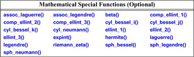
If you don’t know these functions, you are unlikely to need them.
40.4. complex Numbers
The standard library provides complex number types complex<float>, complex<double>, and complex<long double>. A complex<Scalar> where Scalar is some other type supporting the usual arithmetic operations usually works but is not guaranteed to be portable.
template<typename Scalar>
class complex {
// a complex is a pair of scalar values, basically a coordinate pair
Scalar re, im;
public:
complex(const Scalar & r = Scalar{}, const Scalar & i = Scalar{}) :re(r), im(i) { }
Scalar real() const { return re; } // real part
void real(Scalar r) { re=r; }
Scalar imag() const { return im; } // imaginary part
void imag(Scalar i) { im = i; }
template<typename X>
complex(const complex<X>&);
complex<T>& operator=(const T&);
complex& operator=(const complex&);
template<typename X>
complex<T>& operator=(const complex<X>&);
complex<T>& operator+=(const T&);
template<typename X>
complex<T>& operator+=(const complex<X>&);
// similar for operators -=, *=, /=
};
The standard-library complex does not protect against narrowing:
complex<float> z1 = 1.33333333333333333; // narrows
complex<double> z2 = 1.33333333333333333;// narrows
z1=z2; // narrows
To protect against accidental narrowing, use {} initialization:
complex<float> z3 {1.33333333333333333}; // error: narrowing conversion
In addition to the members of complex, <complex> offers a host of useful operations:
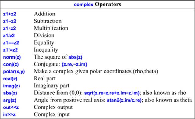
The standard mathematical functions (§40.3) are also available for complex numbers. Note that complex does not provide < or %. For more details, see §18.3.
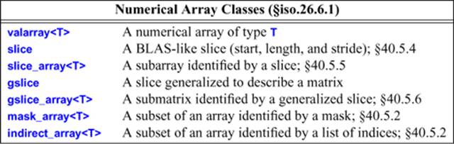
40.5. A Numerical Array: valarray
Much numeric work relies on relatively simple single-dimensional vectors of floating-point values. In particular, such vectors are well supported by high-performance machine architectures, libraries relying on such vectors are in wide use, and very aggressive optimization of code using such vectors is considered essential in many fields. The valarray from <valarray> is a single-dimensional numerical array. It provides the usual numeric vector arithmetic operations for an array type plus support for slices and strides:
The fundamental idea of valarray was to provide Fortran-like facilities for dense multidimensional arrays with Fortran-like opportunities for optimization. This can only be achieved with the active support of compiler and optimization suppliers and the addition of more library support on top of the very basic facilities provided by valarray. So far, that has not happened for all implementations.
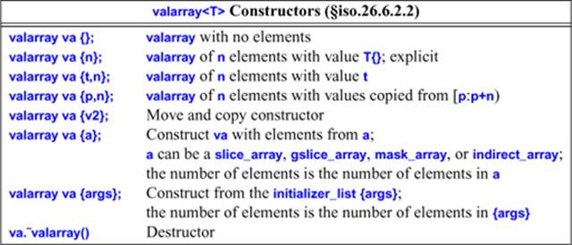
40.5.1. Constructors and Assignments
The valarray constructors allow us to initialize valarrays from the auxiliary numeric array types and from single values:
For example:
valarray<double> v0; // placeholder, we can assign to v0 later
valarray<float> v1(1000); // 1000 elements with value float()==0.0F
valarray<int> v2(–1,2000); // 2000 elements with value –1
valarray<double> v3(100,9.8064); // bad mistake: floating-point valarray size
valarray<double> v4 = v3; // v4 has v3.size() elements
valarray<int> v5 {–1,2000}; // two elements
In the two-argument constructors, the value comes before the number of elements. This differs from the convention for standard containers (§31.3.2).
The number of elements of an argument valarray to a copy constructor determines the size of the resulting valarray.
Most programs need data from tables or input. In addition to initializer lists, this is supported by a constructor that copies elements from a built-in array. For example:
void f(const int* p, int n)
{
const double vd[] = {0,1,2,3,4};
const int vi[] = {0,1,2,3,4};
valarray<double> v1{vd,4}; // 4 elements: 0,1,2,3
valarray<double> v2{vi,4}; // type error: vi is not pointer to double
valarray<double> v3{vd,8}; // undefined: too few elements in initializer
valarray<int> v4{p,n}; // p had better point to at least n ints
}
The valarray and its auxiliary facilities were designed for high-speed computing. This is reflected in a few constraints on users and by a few liberties granted to implementers. Basically, an implementer of valarray is allowed to use just about every optimization technique you can think of. The valarray operations are assumed to be free of side effects (except on their explicit arguments, of course), valarrays are assumed to be alias free, and the introduction of auxiliary types and the elimination of temporaries is allowed as long as the basic semantics are maintained. There is no range checking. The elements of a valarray must have the default copy semantics (§8.2.6).
Assignment can be with another valarray, a scalar, or a subset of a valarray:
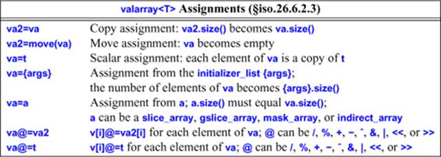
A valarray can be assigned to another of the same size. As one would expect, v1=v2 copies every element of v2 into its corresponding position in v1. If valarrays have different sizes, the result of assignment is undefined.
In addition to this conventional assignment, it is possible to assign a scalar to a valarray. For example, v=7 assigns 7 to every element of the valarray v. This may be surprising to some programmers and is best understood as an occasionally useful degenerate case of the operator assignment operations. For example:
valarray<int> v {1,2,3,4,5,6,7,8};
v *= 2; // v=={2,4,6,10,12,14,16}
v = 7; // v=={7,7,7,7,7,7,7,7}
40.5.2. Subscripting
Subscripting can be used to select an element of a valarray or a subset of its elements:
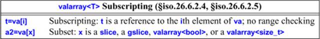
Each operator[] returns a subset of the elements from a valarray. The return type (the type of the object representing the subset) depends on the argument type.
For const arguments, the result contains copies of elements. For non-const arguments, the result holds references to elements. Since C++ doesn’t directly support arrays of references (e.g., we can’t say valarray<int&>), the implementation will somehow simulate this. This can be done efficiently. An exhaustive list, with examples (based on §iso.26.6.2.5), is in order. In each case, the subscript describes the elements to be returned, and v1 must be a vallaray with an appropriate length and element type:
• A slice of a const valarray:
valarray<T> operator[](slice) const;// copy of elements
// ...
const valarray<char> v0 {"abcdefghijklmnop",16};
valarray<char> v1 {v0[slice(2,5,3)]}; // {"cfilo",5}
• A slice of a non-const valarray:
slice_array<T> operator[](slice); // references to elements
// ...
valarray<char> v0 {"abcdefghijklmnop",16};
valarray<char> v1 {"ABCDE",5};
v0[slice(2,5,3)] = v1; // v0=={"abAdeBghCjkDmnEp",16}
• A gslice of a const valarray:
valarray<T> operator[](const gslice&) const; // copies of elements
// ...
const valarray<char> v0 {"abcdefghijklmnop",16};
const valarray<size_t> len {2,3};
const valarray<size_t> str {7,2};
valarray<char> v1 {v0[gslice(3,len,str)]}; // v1=={"dfhkmo",6}
• A gslice of a non-const valarray:
gslice_array<T> operator[](const gslice&); // references to elements
// ...
valarray<char> v0 {"abcdefghijklmnop",16};
valarray<char> v1 {"ABCDE",5};
const valarray<size_t> len {2,3};
const valarray<size_t> str {7,2};
v0[gslice(3,len,str)] = v1; // v0=={"abcAeBgCijDlEnFp",16}
• A valarray<bool> (a mask) of a const valarray:
valarray<T> operator[](const valarray<bool>&) const; // copies of elements
// ...
const valarray<char> v0 {"abcdefghijklmnop",16};
const bool vb[] {false, false, true, true, false, true};
valarray<char> v1 {v0[valarray<bool>(vb, 6)]}; // v1=={"cdf",3}
• A valarray<bool> (a mask) of a non-const valarray:
mask_array<T> operator[](const valarray<bool>&); // references to elements
// ...
valarray<char> v0 {"abcdefghijklmnop", 16};
valarray<char> v1 {"ABC",3};
const bool vb[] {false, false, true, true, false, true};
v0[valarray<bool>(vb,6)] = v1; // v0=={"abABeCghijklmnop",16}
• A valarray<size_t> (a set of indices) of a const valarray:
valarray<T> operator[](const valarray<size_t>&) const; // references to elements
// ...
const valarray<char> v0 {"abcdefghijklmnop",16};
const size_t vi[] {7, 5, 2, 3, 8};
valarray<char> v1 {v0[valarray<size_t>(vi,5)]}; // v1=={"hfcdi",5}
• A valarray<size_t> (a set of indices) of a non-const valarray:
indirect_array<T> operator[](const valarray<size_t>&); // references to elements
// ...
valarray<char> v0 {"abcdefghijklmnop",16};
valarray<char> v1 {"ABCDE",5};
const size_t vi[] {7, 5, 2, 3, 8};
v0[valarray<size_t>(vi,5)] {v1}; // v0=={"abCDeBgAEjklmnop",16}
Note that subscripting with a mask (a valarray<bool>) yields a mask_array, and subscripting with a set of indices (a valarray<size_t>) yields an indirect_array.
40.5.3. Operations
The purpose of valarray is to support computation, so a host of basic numerical operations are directly supported:
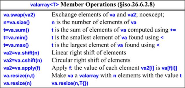
There is no range checking: the effect of using a function that tries to access an element of an empty valarray is undefined.
Note that resize() does not retain any old values.
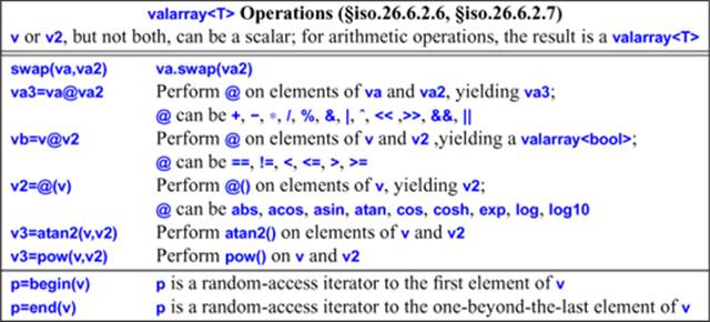
The binary operations are defined for valarrays and for combinations of a valarray and its scalar type. A scalar type is treated as a valarray of the right size with every element having the scalar’s value. For example:
void f(valarray<double>& v, valarray<double>& v2, double d)
{
valarray<double> v3 = v*v2; // v3[i] = v[i]*v2[i] for all i
valarray<double> v4 = v*d; // v4[i] = v[i]*d for all i
valarray<double> v5 = d*v2; // v5[i] = d*v2[i] for all i
valarray<double> v6 = cos(v); // v6[i] = cos(v[i]) for all i
}
These vector operations all apply their operations to each element of their operand(s) in the way indicated by the * and cos() examples. Naturally, an operation can be used only if the corresponding operation is defined for the scalar type. Otherwise, the compiler will issue an error when trying to specialize the operator or function.
Where the result is a valarray, its length is the same as its valarray operand. If the lengths of the two arrays are not the same, the result of a binary operator on two valarrays is undefined.
These valarray operations return new valarrays rather than modifying their operands. This can be expensive, but it doesn’t have to be when aggressive optimization techniques are applied.
For example, if v is a valarray, it can be scaled like this: v*=0.2, and this: v/=1.3. That is, applying a scalar to a vector means applying the scalar to each element of the vector. As usual, *= is more concise than a combination of * and = (§18.3.1) and easier to optimize.
Note that the non-assignment operations construct a new valarray. For example:
double incr(double d) { return d+1; }
void f(valarray<double>& v)
{
valarray<double> v2 = v.apply(incr); // produce incremented valarray
// ...
}
This does not change the value of v. Unfortunately, apply() does not accept a function object (§3.4.3, §11.4) as an argument.
The logical and cyclic shift functions, shift() and cshift(), return a new valarray with the elements suitably shifted and leave the original one unchanged. For example, the cyclic shift v2=v.cshift(n) produces a valarray so that v2[i]==v[(i+n)%v.size()]. The logical shift v3=v.shift(n)produces a valarray so that v3[i] is v[i+n] if i+n is a valid index for v. Otherwise, the result is the default element value. This implies that both shift() and cshift() shift left when given a positive argument and right when given a negative argument. For example:
void f()
{
int alpha[] = { 1, 2, 3, 4, 5 ,6, 7, 8 };
valarray<int> v(alpha,8); // 1, 2, 3, 4, 5, 6, 7, 8
valarray<int> v2 = v.shift(2); // 3, 4, 5, 6, 7, 8, 0, 0
valarray<int> v3 = v<<2; // 4, 8, 12, 16, 20, 24, 28, 32
valarray<int> v4 = v.shift(–2); // 0, 0, 1, 2, 3, 4, 5, 6
valarray<int> v5 = v>>2; // 0, 0, 0, 1, 1, 1, 1, 2
valarray<int> v6 = v.cshift(2); // 3, 4, 5, 6, 7, 8, 1, 2
valarray<int> v7 = v.cshift(–2); // 7, 8, 1, 2, 3, 4, 5, 6
}
For valarrays, >> and << are bit shift operators, rather than element shift operators or I/O operators. Consequently, <<= and >>= can be used to shift bits within elements of an integral type. For example:
void f(valarray<int> vi, valarray<double> vd)
{
vi <<= 2; // vi[i]<<=2 for all elements of vi
vd <<= 2; // error: shift is not defined for floating-point values
}
All of the operators and mathematical functions on valarrays can also be applied to slice_arrays (§40.5.5), gslice_arrays (§40.5.6), mask_arrays (§40.5.2), indirect_arrays (§40.5.2), and combinations of these types. However, an implementation is allowed to convert an operand that is not a valarray to a valarray before performing a required operation.
40.5.4. Slices
A slice is an abstraction that allows us to manipulate a one-dimensional array (e.g., a built-in array, a vector, or a valarray) efficiently as a matrix of arbitrary dimension. It is the key notion of Fortran vectors and of the BLAS (Basic Linear Algebra Subprograms) library, which is the basis for much numeric computation. Basically, a slice is every nth element of some part of an array:
class std::slice {
// starting index, a length, and a stride
public:
slice(); // slice{0,0,0}
slice(size_t start, size_t size, size_t stride);
size_t start() const; // index of first element
size_t size() const; // number of elements
size_t stride() const; // element n is at start()+n*stride()
};
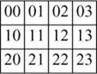
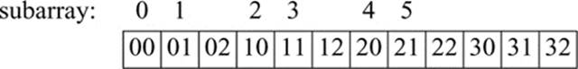
A stride is the distance (in number of elements) between two elements of the slice. Thus, a slice describes a mapping of non-negative integers into indices. The number of elements (the size()) doesn’t affect the mapping (addressing) but allows us to find the end of a sequence. This mapping can be used to simulate two-dimensional arrays within a one-dimensional array (such as valarray) in an efficient, general, and reasonably convenient way. Consider a 3-by-4 matrix (three rows, each with four elements):
valarray<int> v {
{00,01,02,03}, // row 0
{10,11,12,13}, // row 1
{20,21,22,23} // row 2
};
or graphically:
Following the usual C/C++ conventions, the valarray is laid out in memory with row elements first (row-major order) and contiguous:
for (int x : v) cout << x << ' ' ;
This produces:
0 1 2 3 10 11 12 13 20 21 22 23
or graphically:
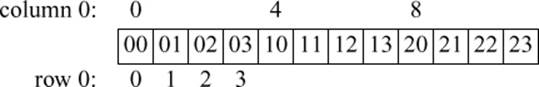
Row x is described by slice(x*4,4,1). That is, the first element of row x is the x*4th element of the vector, the next element of the row is the (x*4+1)th, etc., and there are 4 elements in each row. For example, slice{0,4,1} describes the first row of v (row 0): 00, 01, 02, 03, and slice{1,4,1}describes the second row (row 1).
Column y is described by slice(y,3,4). That is, the first element of column y is the yth element of the vector, the next element of the column is the (y+4)th, etc., and there are 3 elements in each column. For example, slice{0,3,4} describes the first column (column 0): 00, 10, 20, andslice{1,3,4} describes the second column (column 1).
In addition to its use for simulating two-dimensional arrays, a slice can describe many other sequences. It is a fairly general way of specifying very simple sequences. This notion is explored further in §40.5.6.
One way of thinking of a slice is as an odd kind of iterator: a slice allows us to describe a sequence of indices for a valarray. We could build an STL-style iterator based on that:
template<typename T>
class Slice_iter {
valarray<T>*v;
slice s;
size_t curr; // index of current element
T& ref(size_t i) const { return (*v)[s.start()+i*s.stride()]; }
public:
Slice_iter(valarray<T>*vv, slice ss, size_t pos =0)
:v{vv}, s{ss}, curr{0} { }
Slice_iter end() const { return {this,s,s.size()}; }
Slice_iter& operator++() { ++curr; return *this; }
Slice_iter operator++(int) { Slice_iter t = *this; ++curr; return t; }
T& operator[](size_t i) { return ref(i); } // C-style subscript
T& operator()(size_t i) { return ref(i); } // Fortran-style subscript
T& operator*() { return ref(curr); } // current element
bool operator==(const Slice_iter& q) const
{
return curr==q.curr && s.stride()==q.s.stride() && s.start()==q.s.start();
}
bool operator!=(const Slice_iter& q) const
{
return !(*this==q);
}
bool operator<(const Slice_iter& q) const
{
return curr<q.curr && s.stride()==q.s.stride() && s.start()==q.s.start();
};
}
Since a slice has a size, we could even provide range checking. Here, I have taken advantage of slice::size() to provide an end() operation to provide an iterator for the one-past-the-end element of the slice.
Since a slice can describe either a row or a column, the Slice_iter allows us to traverse a valarray by row or by column.
40.5.5. slice_array
From a valarray and a slice, we can build something that looks and feels like a valarray but is really simply a way of referring to the subset of the array described by the slice.
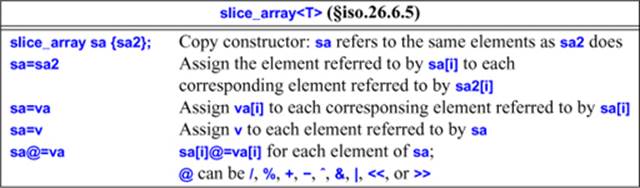
A user cannot directly create a slice_array. Instead, the user subscripts a valarray to create a slice_array for a given slice. Once the slice_array is initialized, all references to it indirectly go to the valarray for which it is created. For example, we can create something that represents every second element of an array like this:
void f(valarray<double>& d)
{
slice_array<double>& v_even = d[slice(0,d.size()/2+d.size()%2,2)];
slice_array<double>& v_odd = d[slice(1,d.size()/2,2)];
v_even *= v_odd; // multiply element pairs and store results in even elements
v_odd = 0; // assign 0 to every odd element of d
}
A slice_array can be copied. For example:
slice_array<double> row(valarray<double>& d, int i)
{
slice_array<double> v = d[slice(0,2,d.size()/2)];
// ...
return d[slice(i%2,i,d.size()/2)];
}
40.5.6. Generalized Slices
A slice (§29.2.2, §40.5.4) can describe a row or a column of an n-dimensional array. However, sometimes we need to extract a subarray that is not a row or a column. For example, we might want to extract the 3-by-2 matrix from the top-left corner of a 4-by-3 matrix:
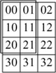
Unfortunately, these elements are not allocated in a way that can be described by a single slice:
A gslice is a “generalized slice” that contains (almost) the information from n slices:
class std::gslice {
// instead of 1 stride and one size like slice, gslice holds n strides and n sizes
public:
gslice();
gslice(size_t sz, const valarray<size_t>& lengths, const valarray<size_t>& strides);
size_t start() const; // index of first element
valarray<size_t> size() const; // number of elements in dimension
valarray<size_t> stride() const; // stride for index[0], index[1], ...
};
The extra values allow a gslice to specify a mapping between n integers and an index to be used to address elements of an array. For example, we can describe the layout of the 3-by-2 matrix by a pair of (length,stride) pairs:
size_t gslice_index(const gslice& s, size_t i, size_t j) // max (i,j) to their corresponding index
{
return s.start()+i*s.stride()[0]+j*s.stride()[1];
}
valarray<size_t> lengths {2,3};// 2 elements in the first dimension
// 3 elements in the second dimension
valarray<size_t> strides {3,1}; // 3 is the stride for the first index
// 1 is the stride for the second index
void f()
{
gslice s(0,lengths,strides);
for (int i=0; i<3; ++i) // for each row
for (int j=0; j<2; ++j) // for each element in row
cout << "(" << i << "," << j << ")–>" << gslice_index(s,i,j) << "; "; // print mapping
}
This prints:
(0,0)–>0; (0,1)–>1; (1,0)–>3; (1,1)–>4; (2,0)–>6; (2,1)–>7
In this way, a gslice with two (length,stride) pairs describes a subarray of a two-dimensional array, a gslice with three (length,stride) pairs describes a subarray of a three-dimensional array, etc. Using a gslice as the index of a valarray yields a gslice_array consisting of the elements described by the gslice. For example:
void f(valarray<float>& v)
{
gslice m(0,lengths,strides);
v[m] = 0; // assign 0 to v[0],v[1],v[3],v[4],v[6],v[7]
}
The gslice_array offers the same set of members as slice_array (§40.5.5). A gslice_array is the result of using a gslice as the subscript of a valarray (§40.5.2).
40.6. Generalized Numerical Algorithms
In <numeric>, the standard library provides a few generalized numeric algorithms in the style of the non-numeric algorithms from <algorithm> (Chapter 32). These algorithms provide general versions of common operations on sequences of numerical values:
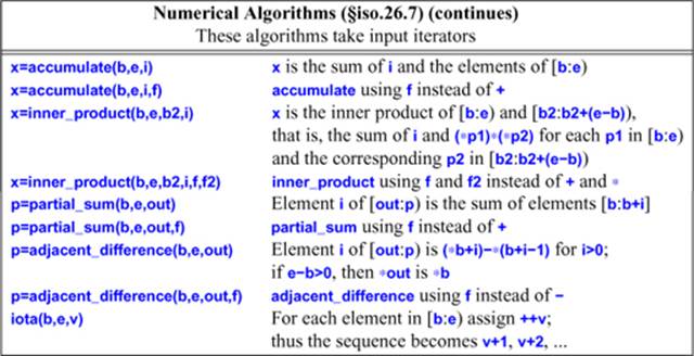
These algorithms generalize common operations such as computing a sum by letting them apply to all kinds of sequences and by making the operation applied to elements of those sequences a parameter. For each algorithm, the general version is supplemented by a version applying the most common operator for that algorithm.
40.6.1. accumulate()
The simple version of accumulate() adds elements of a sequence using their + operator:
template<typename In, typename T>
T accumulate(In first, In last, T init)
{
for (; first!=last; ++first) // for all elements in [first:last)
init = init + *first; // plus
return init;
}
It can be used like this:
void f(vector<int>& price, list<float>& incr)
{
int i = accumulate(price.begin(),price.end(),0); // accumulate in int
double d = 0;
d = accumulate(incr.begin(),incr.end(),d); // accumulate in double
int prod = accumulate(price.begin,price.end(),1,[](int a, int b) { return a*b; });
// ...
}
The type of the initial value passed determines the return type.
We can provide an initial value and an operation for “combining elements” as arguments to accumulate(), so accumulate() is not all about addition.
Extracting a value from a data structure is common operation for accumulate(). For example:
struct Record {
// ...
int unit_price;
int number_of_units;
};
long price(long val, const Record& r)
{
return val + r.unit_price * r.number_of_units;
}
void f(const vector<Record>& v)
{
cout << "Total value: " << accumulate(v.begin(),v.end(),0,price) << '\n';
}
Operations similar to accumulate are called reduce, reduction, and fold in some communities.
40.6.2. inner_product()
Accumulating from a sequence is very common, and accumulating from a pair of sequences is not uncommon:
template<typename In, typename In2, typename T>
T inner_product(In first, In last, In2 first2, T init)
{
while (first != last)
init = init + *first++ **first2++;
return init;
}
template<typename In, typename In2, typename T, typename BinOp, typename BinOp2>
T inner_product(In first, In last, In2 first2, T init, BinOp op, BinOp2 op2)
{
while (first != last)
init = op(init,op2(*first++,*first2++));
return init;
}
As usual, only the beginning of the second input sequence is passed as an argument. The second input sequence is assumed to be at least as long as the first.
The key operation in multiplying a Matrix by a valarray is an inner_product:
valarray<double> operator*(const Matrix& m, valarray<double>& v)
{
valarray<double> res(m.dim2());
for (size_t i=0; i<m.dim2(); i++) {
auto& ri = m.row(i);
res[i] = inner_product(ri,ri.end(),&v[0],double(0));
}
return res;
}
valarray<double> operator*(valarray<double>& v, const Matrix& m)
{
valarray<double> res(m.dim1());
for (size_t i=0; i<m.dim1(); i++) {
auto& ci = m.column(i);
res[i] = inner_product(ci,ci.end(),&v[0],double(0));
}
return res;
}
Some forms of inner_product are referred to as “dot product.”
40.6.3. partial_sum() and adjacent_difference()
The partial_sum() and adjacent_difference() algorithms are inverses of each other and deal with the notion of incremental change.
Given a sequence a, b, c, d, etc., adjacent_difference() produces a, b–a, c–b, d–c, etc.
Consider a vector of temperature readings. We could transform it into a vector of temperature changes like this:
vector<double> temps;
void f()
{
adjacent_difference(temps.begin(),temps.end(),temps.begin());
}
For example, 17, 19, 20, 20, 17 turns into 17, 2, 1, 0, –3.
Conversely, partial_sum() allows us to compute the end result of a set of incremental changes:
template<typename In, typename Out, typename BinOp>
Out partial_sum(In first, In last, Out res, BinOp op)
{
if (first==last) return res;
*res = *first;
T val = *first;
while (++first != last) {
val = op(val,*first);
*++res = val;
}
return ++res;
}
template<typename In, typename Out>
Out partial_sum(In first, In last, Out res)
{
return partial_sum(first,last,res,plus); // use std::plus (§33.4)
}
Given a sequence a, b, c, d, etc., partial_sum() produces a, a+b, a+b+c, a+b+c+d, etc. For example:
void f()
{
partial_sum(temps.begin(),temps.end(),temps.begin());
}
Note the way partial_sum() increments res before assigning a new value through it. This allows res to be the same sequence as the input; adjacent_difference() behaves similarly. Thus,
partial_sum(v.begin(),v.end(),v.begin());
turns the sequence a, b, c, d into a, a+b, a+b+c, a+b+c+d, and
adjacent_difference(v.begin(),v.end(),v.begin());
reproduces the original value. Thus, partial_sum() turns 17, 2, 1, 0, –3 back into 17, 19, 20, 20, 17.
For people who think of temperature differences as a boring detail of meteorology or science lab experiments, I note that analyzing changes in stock prices or sea levels involves exactly the same two operations. These operations are useful for analyzing any series of changes.
40.6.4. iota()
A call iota(b,e,n) assigns n+i to the ith element of [b:e). For example:
vector<int> v(5);
iota(v.begin(),v.end(),50);
vector<int> v2 {50,51,52,53,54}
if (v!=v2)
error("complain to your library vendor");
The name iota is the Latin spelling of the Greek letter ![]() , which was used for that function in APL.
, which was used for that function in APL.
Do not confuse iota() with the non-standard, but not uncommon, itoa() (int-to-alpha; §12.2.4).
40.7. Random Numbers
Random numbers are essential to many applications, such as simulations, games, sampling-based algorithms, cryptography, and testing. For example, we might want to choose the TCP/IP address for a router simulation, decide whether a monster should attack or scratch its head, or generate a set of values for testing a square root function. In <random>, the standard library defines facilities for generating (pseudo-)random numbers. These random numbers are sequences of values produced according to mathematical formulas, rather than unguessable (“truly random”) numbers that could be obtained from a physical process, such as radioactive decay or solar radiation. If the implementation has such a truly random device, it will be represented as a random_device (§40.7.1).
Four kinds of entities are provided:
• A uniform random number generator is a function object returning unsigned integer values such that each value in the range of possible results has (ideally) equal probability of being returned.
• A random number engine (an engine) is a uniform random number generator that can be created with a default state E{} or with a state determined by a seed E{s}.
• A random number engine adaptor (an adaptor) is a random number engine that takes values produced by some other random number engine and applies an algorithm to those values in order to deliver a sequence of values with different randomness properties.
• A random number distribution (a distribution) is a function object returning values that are distributed according to an associated mathematical probability density function p(z) or according to an associated discrete probability function P(zi).
For details see §iso.26.5.1.
In simpler terms, the users’ terms, a random number generator is an engine plus a distribution. The engine produces a uniformly distributed sequence of values, and the distribution bends those into the desired shape (distribution). That is, if you take lots of numbers from a random number generator and draw them, you should get a reasonably smooth graph of their distribution. For example, binding a normal_distribution to the default_random_engine gives me a random number generator that produces a normal distribution:
auto gen = bind(normal_distribution<double>{15,4.0},default_random_engine{});
for (int i=0; i<500; ++i) cout << gen();
The standard-library function bind() makes a function object that will invoke its first argument given its second argument (§33.5.1).
Using ASCII graphics (§5.6.3), I got:
3 **
4 *
5 *****
6 ****
7 ****
8 ******
9 ************
10 ***************************
11 ***************************
12 **************************************
13 **********************************************************
14 ***************************************************
15 *******************************************************
16 ********************************
17 **************************************************
18 *************************************
19 **********************************
20 ***************
21 ************
22 ************
23 *******
24 *****
25 ****
26 *
27 *
Most of the time, most programmers just need a simple uniform distribution of integers or floating-point numbers in a given range. For example:
void test()
{
Rand_int ri {10,20}; // uniform distribution of ints in [10:20)
Rand_double rd {0,0.5}; // uniform distribution of doubles in [0:0.5)
for (int i=0; i<100; ++i)
cout << ri() << ' ';
for (int i=0; i<100; ++i)
cout << rd() << ' ';
}
Unfortunately, Ran_int and Rand_double are not standard classes, but they are easy to build:
class Rand_int {
Rand_int(int lo, int hi) : p{lo,hi} { } // store the parameters
int operator()() const { return r(); }
private:
uniform_int_distribution<>::param_type p;
auto r = bind(uniform_int_distribution<>{p},default_random_engine{});
};
I store the parameters using the distribution’s standard param_type alias (§40.7.3) so that I can use auto to avoid having to name the result of the bind().
Just for variation, I use a different technique for Rand_double:
class Rand_double {
public:
Rand_double(double low, double high)
:r(bind(uniform_real_distribution<>(low,high),default_random_engine())) { }
double operator()() { return r(); }
private:
function<double()> r;
};
One important use of random numbers is for sampling algorithms. In such algorithms we need to choose a sample of some size from a much larger population. Here is algorithm R (the simplest algorithm) from a famous old paper [Vitter,1985]:
template<typename Iter, typename Size, typename Out, typename Gen>
Out random_sample(Iter first, Iter last, Out result, Size n, Gen&& gen)
{
using Dist = uniform_int_distribution<Size>;
using Param = typename Dist::param_type;
// Fill the reservoir and advance first:
copy(first,n,result);
advance(first,n);
// Sample the remaining values in [first+n:last) by selecting a random
// number r in the range [0:k], and, if r<n, replace it.
// k increases with each iteration, making the probability smaller.
// For random access iterators, k = i-first (assuming we increment i and not first).
Dist dist;
for (Size k = n; first!=last; ++first,++k) {
Size r = dist(gen,Param{0,k});
if(r < n)
*(result + r) = *first;
}
return result;
}
40.7.1. Engines
A uniform random number generator is a function object that produces an approximately uniformly distributed sequence of values of its result_type:
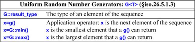
A random number engine is a uniform random number generator with additional properties to make it widely useful:
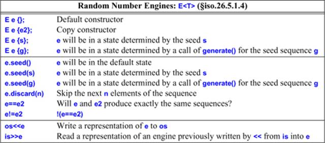
A seed is a value in the range [0:232) that can be used to initialize a particular engine. A seed sequence, g, is an object that provides a function g.generate(b,e) that when called fills [b:e) with newly generated seeds (§iso.26.5.1.2).
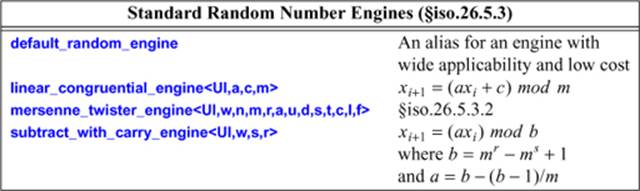
The UI parameter for a standard random number engine must be an unsigned integer type. For linear_congruential_engine<UI,a,c,m>, if the modulus m is 0, the value numeric_limits<result_type>::max()+1 is used. For example, this writes out the index of the first repetition of a number:
map<int,int> m;
linear_congruential_engine<unsigned int,17,5,0> linc_eng;
for (int i=0; i<1000000; ++i)
if (1<++m[linc_eng()]) cout << i << '\n';
I was lucky; the parameters were not too bad and I got no duplicate values. Try <unsigned int,16,5,0> instead and see the difference. Use the default_random_engine unless you have a real need and know what you are doing.
A random number engine adaptor takes a random number engine as an argument and produces a new random number engine with different randomness properties.
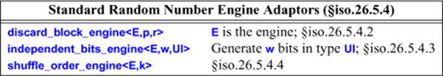
For example:
independent_bits_engine<default_random_engine,4,unsigned int> ibe;
for (int i=0; i<100; ++i)
cout << '0'+ibe() << ' ';
This will produce 100 numbers in the range [48:63] ([’0’:’0’+24-1)).
A few aliases are defined for useful engines:
using minstd_rand0 = linear_congruential_engine<uint_fast32_t, 16807, 0, 2147483647>;
using minstd_rand = linear_congruential_engine<uint_fast32_t, 48271, 0, 2147483647>;
using mt19937 = mersenne_twister_engine<uint_fast32_t, 32,624,397,
31,0x9908b0df,
11,0xffffffff,
7,0x9d2c5680,
15,0xefc60000,
18,1812433253>
using mt19937_64 = mersenne_twister_engine<uint_fast64_t, 64,312,156,
31,0xb5026f5aa96619e9,
29, 0x5555555555555555,
17, 0x71d67fffeda60000,
37, 0xfff7eee000000000,
43, 6364136223846793005>;
using ranlux24_base = subtract_with_carry_engine<uint_fast32_t, 24, 10, 24>;
using ranlux48_base = subtract_with_carry_engine<uint_fast64_t, 48, 5, 12>;
using ranlux24 = discard_block_engine<ranlux24_base, 223, 23>;
using ranlux48 = discard_block_engine<ranlux48_base, 389, 11>;
using knuth_b = shuffle_order_engine<minstd_rand0,256>;
40.7.2. Random Device
If an implementation is able to offer a truly random number generator, that source of random numbers is presented as a uniform random number generator called random_device:
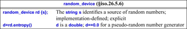
Think of s as the name of a random number source, such as a Geiger counter, a Web service, or a file/device containing the record of a truly random source. The entropy() is defined as
![]()
for a device with n states whose respective probabilities are P0,..., Pn–1. The entropy is an estimate of the randomness, the degree of unpredictability, of the generated numbers. In contrast to thermodynamics, high entropy is good for random numbers because that means that it is hard to guess subsequent numbers. The formula reflects the result of repeatedly throwing a perfect n-sided dice.
The random_device is intended to be useful for cryptograpic applications, but it would be against all rules of that kind of application to trust an implementation of random_device without first studying it closely.
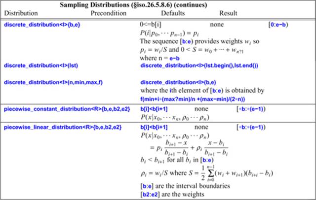
40.7.3. Distributions
A random number distribution is a function object that, when called with a random number generator argument, produces a sequence of values of its result_type:
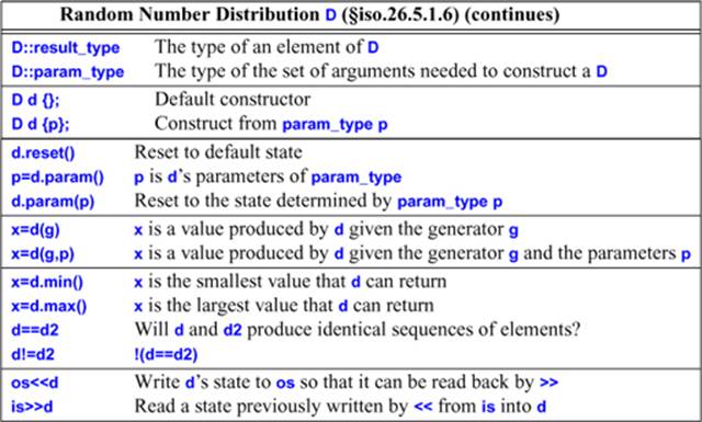
In the following tables, a template argument R means a real is required in the mathematical formula and double is the default. An I means that an integer is required and int is the default.
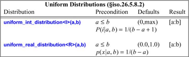
The precondition field specifies requirements on the distribution arguments. For example:
uniform_int_distribution<int> uid1 {1,100}; // OK
uniform_int_distribution<int> uid2 {100,1}; // error: a>b
The default field specifies default arguments. For example:
uniform_real_distribution<double> urd1 {}; // use a==0.0 and b==1.0
uniform_real_distribution<double> urd2 {10,20}; // use a==10.0 and b==20.0
uniform_real_distribution<> urd3 {}; // use double and a==0.0 and b==1.0
The result field specifies the range of the results. For example:
uniform_int_distribution<> uid3 {0,5};
default_random_engine e;
for (int i=0; i<20; ++i)
cout << uid3(e) << ' ';
The range for uniform_int_distribution is closed, and we see the six possible values:
2 0 2 5 4 1 5 5 0 1 1 5 0 0 5 0 3 4 1 4
For uniform_real_distribution, as for all other distributions with floating-point results, the range is half-open.
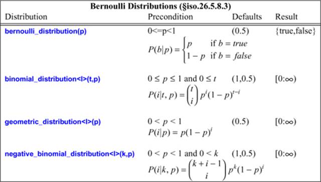
Bernoulli distributions reflect sequences of tosses of coins with varying degrees of loading:
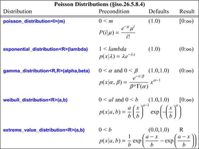
Poisson distributions express the probability of a given number of events occurring in a fixed interval of time and/or space:
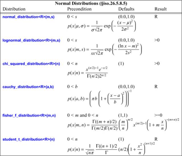
Normal distributions map real values into real values. The simplest is the famous “bell curve” that distributes values symmetrically around a peak (mean) with the distance of elements from the mean being controlled by a standard deviation parameter:
To get a feeling for these distributions, look at graphical representations for a variety of parameters. Such representations are easily generated and even more easily found on the Web.
Sampling distributions map integers into a specific range according to their probability density function P:
40.7.4. C-Style Random Numbers
In <cstdlib> and <stdlib.h>, the standard library provides a simple basis for the generation of random numbers:
#define RAND_MAX implementation_defined /* large positive integer */
int rand(); // pseudo-random number between 0 and RAND_MAX
void srand(unsigned int i); // seed random number generator by i
Producing a good random number generator isn’t easy, and unfortunately not all systems deliver a good rand(). In particular, the low-order bits of a random number are often suspect, so rand()%n is not a good portable way of generating a random number between 0 and n–1. Often,int((double(rand())/RAND_MAX)*n) gives acceptable results. However, for serious applications, generators based on uniform_int_distribution (§40.7.3) will give more reliable results.
A call srand(s) starts a new sequence of random numbers from the seed, s, given as argument. For debugging, it is often important that a sequence of random numbers from a given seed be repeatable. However, we often want to start each real run with a new seed. In fact, to make games unpredictable, it is often useful to pick a seed from the environment of a program. For such programs, some bits from a real-time clock often make a good seed.
40.8. Advice
[1] Numerical problems are often subtle. If you are not 100% certain about the mathematical aspects of a numerical problem, either take expert advice, experiment, or do both; §29.1.
[2] Use variants of numeric types that are appropriate for their use; §40.2.
[3] Use numeric_limits to check that the numeric types are adequate for their use; §40.2.
[4] Specialize numeric_limits for a user-defined numeric type; §40.2.
[5] Prefer numeric_limits over limit macros; §40.2.1.
[6] Use std::complex for complex arithmetic; §40.4.
[7] Use {} initialization to protect against narrowing; §40.4.
[8] Use valarray for numeric computation when run-time efficiency is more important than flexibility with respect to operations and element types; §40.5.
[9] Express operations on part of an array in terms of slices rather than loops; §40.5.5.
[10] Slices is a generally useful abstraction for access of compact data; §40.5.4, §40.5.6.
[11] Consider accumulate(), inner_product(), partial_sum(), and adjacent_difference() before you write a loop to compute a value from a sequence; §40.6.
[12] Bind an engine to a distribution to get a random number generator; §40.7.
[13] Be careful that your random numbers are sufficiently random; §40.7.1.
[14] If you need genuinely random numbers (not just a pseudo-random sequence), use random_device; §40.7.2.
[15] Prefer a random number class for a particular distribution over direct use of rand(); §40.7.4.