Better Business Decisions from Data: Statistical Analysis for Professional Success (2014)

Part VI. Big Data

Chapter 23. Predictive Analytics

It’s Only Arithmetic!

The first step in interrogating the data for a possible relationship is the selection of a limited amount of data, called the training data, from which a model will be developed. The model is an idealized relationship, involving a number of variables, that is suggested by initial examination of the training data or by practical observations. Many different kinds of models are in use, having been drawn from different disciplines. Predictive analytics is essentially a statistical process in that the results obtained are not precise but are expressed in terms of probability. Thus, levels of reliability in terms of confidence limits are a feature. The various statistical methods that we have discussed in previous chapters have their use in setting up proposed models. In addition, techniques from studies of machine learning, artificial intelligence, and neural networks are in use. The development of new and improved models is an active area of research. The following sections are intended to give an indication of the kinds of models that are used and the way in which they work.

Simple Rules

A rule is an “if … then …” statement which may include few or many variables. We could have a rule, for example, that if an applicant for a mortgage is a self-employed plumber aged between 30 and 40 years, then it is 90% certain that he will not default on his payments. Rules are more appropriate when the variables are descriptive, although numerical variables can be dealt with by grouping values within defined limits as in the example quoted.

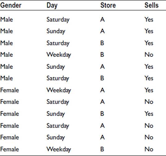
The 1R (One Rule) rule selects one variable from a number of possibilities on the basis of which variable gives the least number of errors. To illustrate the method, we will use the following data, which shows whether a particular item sells or not. We have data for 12 customers, male and female, on different days of the week at two different stores. This is an incredibly small sample but serves to illustrate the procedure:

For each variable, we note the majority result:

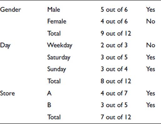
Gender is adopted as the variable for the rule because the number of total successes, 9 out of 12, is the highest of the three. So the rule is that the item sells if the customer is male but not if the customer is female.

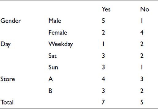
With the use of simple statistics, the approach can be extended to produce several rules from the same data so that the effect of all the variables can be seen (Frank, 2009). The same data is set out differently here:

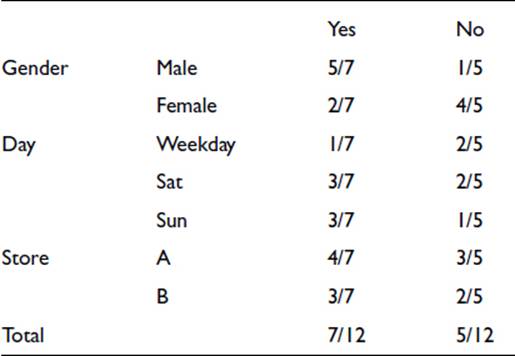
We now express the Yes and No numbers as probabilities. Thus, 5/7, below, is the probability that when a sale takes place the customer is male. The fractions listed in the Total column are the probabilities of getting a sale or not in the whole of the data:

These probabilities allow us to provide a rule for each of the various combinations of the variable levels by using the multiplication rule (the “and” rule) introduced in Chapter 3. For example, if we have a male on a weekday in store A, the relative probability of a sale is

5/7 x 1/7 x 4/7 x 7/12 = 0.034

and the relative probability of no sale is

1/5 x 2/5 x 3/5 x 5/12 = 0.020 .

Note that these are not true probabilities in this form, as the two do not add to unity, but they are in the correct proportion so we can normalize the values to

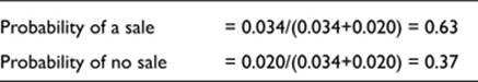
The rule would therefore be that there would on balance be a sale, though the evidence is weak.

To take a further example, a female on a Saturday in store B leads to the following calculation:

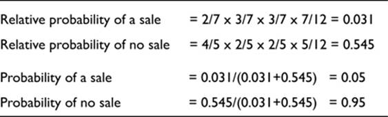
There would be a greater degree of confidence in this rule than in the previous one.

The approach provides us with twelve rules, one for each of the twelve combinations of the levels of the three variables. Some rules will be more reliable than others. If it happens that the data contains contradictory entries, and this is likely in a reasonably large sample, the uncertainty in the derived rules will be greater.

There is a more serious problem with this simple technique. It will be recalled from Chapter 3 that for probabilities to be multiplied together in the “and” rule, the variables must be independent. It is likely that many of the variables in the database are not independent. In the above example it is likely that weekday shoppers are largely female. The effect of dependency between the variables is to bias the result. By multiplying the probability of the sale being to a female customer by the probability that the sale is on a weekday, we could be increasing the effect of the customer being female.

It is evident that a set of data can generate a large number of rules; and because of this, there is a danger of over-fitting. We previously discussed over-fitting in relation to nonlinear regression, where we saw that it is always possible to obtain an equation that produces a curve passing through every point on a graph. Such an equation is of no practical use. Similarly here, we could end up with a set of rules that describes perfectly every situation represented in the training data. But the set of rules would then be merely an alternative representation of the training data and would have achieved nothing.

The usefulness of a rule depends on two characteristics: accuracy and coverage. As we saw above, accuracy can be expressed as the probability that the rule will give a correct result. Coverage indicates the relative occurrence of the rule in the database. In the data presented above, only one quarter of the data involves purchases during weekdays, so the coverage of rules involving such purchases is only 25%. Rules having high accuracy and high coverage are clearly desirable, but low-coverage rules can be extremely useful if each occurrence is very profitable.

More sophisticated methods are available for determining rules. A common feature is that they operate on a bottom-up procedure. The data is split on the basis of the levels of one variable giving two groups, say. A split on the basis of a second variable in a similar way gives four groups.

PRISM is a commercially available system that builds up rules by repeatedly testing and modifying the rule under construction.¹ It starts with a simple “if A then Z” rule, selecting A on the basis of the proportion of correct predictions. Improvement is obtained by selecting B in a similar way, giving “if A and B then Z.” The procedure continues, bringing in C, D, E, etc. as required, until the rule is perfect. The resulting rules are numerous, and some will be contradictory. The ambiguities have to be dealt with, possibly by selecting on the basis of coverage.

Decision Trees

A decision tree is a well-known structure and is popular on account of it being very easy to follow. Figure 23-1 shows a tree built from the data we used in the previous section. At each stage in the tree, the data is separated according to a criterion—in other words, by answering a question. The aim is to ask the right question at each stage so that the data is separated appropriately in order to make useful predictions.

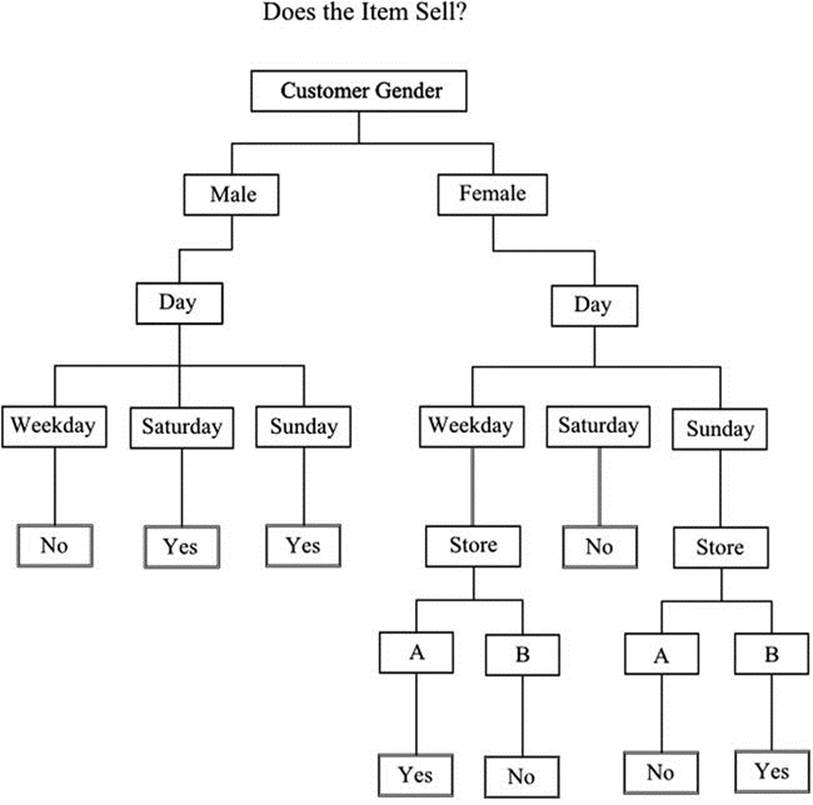
Figure 23-1. A simple decision tree

The key issue, therefore, is the choice of the best question to ask at each stage. Classification and Regression Tree (CART), which is a commonly used method, examines all possible questions and selects the best. The best is the one that decreases the disorder of the data; and for this reason the term entropy, which is a measure of disorder, is used. A complex tree is in effect constructed, but repeated validation at each stage and avoidance of over-fitting result in an efficient structure.

Another method is Chi-squared Automatic Interaction Detector (CHAID). As the name indicates, the Chi-squared test (Chapter 7) is used to decide which questions are to be asked to form the splits in the tree. Contingency tables are set up and, you will recall, the data has to be descriptive. Continuous numerical data can be grouped in categories in order to be dealt with. The trees, unlike the ones resulting from CART, can employ multiple splits, which leads to wider arrangements and eases interpretation.

Decision trees generate rules, but there is a difference between these and the rules obtained by the methods we looked at in the previous section. Decision trees work from the top down, searching for the best possible split at each level. For each record, there will be a rule to cover it and only one rule. In the example shown in Figure 23-1, taking each route from the top down will repeat the records that were used to build the tree. This is, of course, a case of overfitting, justified here in order to show the principle with a small amount of data.

Association

Each record in a database shows association between the variables at the specified values or levels. If we look back at the first record in the example data we used to illustrate the development of rules, we can see how this applies. We had “If male and Saturday and store A, then yes.” Thus we have association between four variables in the record. In fact, we can break down the association to give many more associations in the form of rules:

If male then Saturday

If Saturday then male

If male and Saturday then store A

If male and Saturday then store A and yes

and so on

A total of 50 rules could be stated on the basis of the associations revealed in this single record. This is a very large number; but, of course, it is unlikely that many of the rules would be of practical use. Because so many rules can be generated, it is necessary to have a rationale for weeding out the ones unlikely to be useful and for selecting productive ones.

The selecting is on the basis of accuracy and coverage. Accuracy will show the likelihood of the rule giving the correct answer, and coverage will indicate how often the rule is likely to apply.

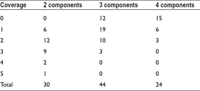
We can use the full list of twelve records from the previous example to show how the procedure is applied. The number of levels included in the data is as follows:

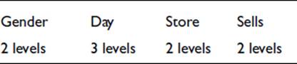
The number of possible two-component groups—e.g., “Male, Saturday”—is 30.

The number of possible three-component groups—e.g., “Male, Saturday, A”—is 44.

The number of possible four-component groups—e.g., “Male, Saturday, A, Yes”—is 24.

Note that these numbers are not readily apparent: They arise from summing the possible combinations of the levels of the variables.

We can reduce the number of groups of interest by considering coverage. Male and Saturday appear in three of the twelve records so coverage is 3/12, or 25%. Similarly, the following values are obtained by comparing the records with the complete set of combinations:

We might decide at this stage that it is worth considering only those groups with a coverage of 4 or 5, and make a further judgment on these on the basis of accuracy. The three selected groups are all two-component, so each group gives us two possible rules. These are as follows:

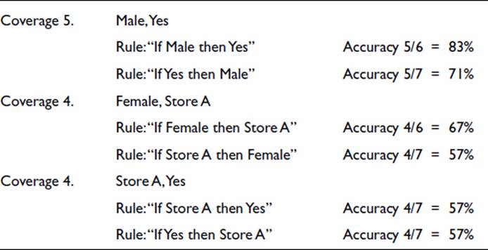
Note that, if we had been considering groups with more components, there would have been many possible rules for each group because of the ways that the members of the group can combine on either side of the if-then statement. We mentioned that just one of the four-component groups gives rise to 50 possible rules.

It is worth pointing out that the rule having the highest accuracy with the maximum coverage—i.e., if the customer is male then the item sells—is the rule that we found using the 1R rule when we discussed simple rules.

It is very laborious working through the coverage of the groups and the accuracy of the rules by hand, even when there are few data—but it is, of course, a simple task for a computer program.

Clustering

Clustering is the grouping of data in such a way that the levels of the variables in each group are more similar than the levels of the corresponding variables in the other groups. Suppliers, for example, could be grouped according to the type of goods supplied, on their location, or on the value of goods supplied. Patients could be grouped according to their various symptoms. If any one of the variables was used for grouping, it is unlikely that the other variables would show an identical grouping. The aim is to establish which variable or combination of variables gives the optimum overall grouping.

Thus the manner of grouping is not decided at the outset. The grouping technique fixes the grouping, and the situation is referred to as unsupervised learning. There is no preconceived pattern to be imposed on the process, and it may not even be evident when the grouping is completed what the logic is that has fixed the optimum outcome. However, a decision has to be made as to how many groups would be desirable. Clearly, without some restriction on number, the optimum arrangement would be an enormous number of groups with one member in each. This would be a case of overfitting and would not serve any useful purpose.

The grouping progresses on the basis of the proximity of one record to another. The proximity is taken to be the distance separating the records. If we think initially of two variables, x and y, a two-dimensional graph would allow the plotting of each record, and the points might show clustering in some regions—small x and large y, say. The distance between each pair of points would be the length of the straight line joining the two points, and this would be a measure of the association. For three variables, we could draw a three-dimensional graph, and the required measures would again be the lengths of the lines joining the points. Although we cannot draw beyond three dimensions, there is no problem mathematically in having an unlimited number of dimensions, to cater for all the variables, and calculating the distances between the various points. The grouping is optimum when the distances within the groups are minimized and the distances between the groups are maximized. The variables, of course, have different units (dollars, weeks, meters, etc.), and an equivalence has to be defined to allow the distances to be calculated. The equivalence could be on the basis of the range of each variable.

Many variations in the iterative routine work toward the optimum grouping. The group centers, which may be initially chosen randomly, are modified according to the resultant calculated distances. Some systems work from an initially defined number of groups and allow subsequent changes to the number. Other systems produce a hierarchy of groups, either starting from a coarse grouping and breaking it down, or starting from the separate records and progressively reducing the number of groups. Although we have referred to an optimum grouping in the discussion, it should be noted that no system can guarantee a perfect unique solution.

Closely related to clustering is the nearest neighbor technique. The concept of proximity in multidimensional space is again used; but rather than attempting to rationalize the data by grouping, the aim is to establish similarities between records to provide predictions. It is thus a form of supervised learning, unlike clustering.

Neural Networks

A neural network is so named because of the similarity to the network of neurons in the brain. The analogy is extended to speaking of the neural network as being able to learn in the way the brain learns, although the analogy should not be taken too far. It is not correct to assume that the neural network is a black box that can simply be fed the data, which it will learn to process and then output the answers. Nonetheless, neural networks emerged from the discipline of artificial intelligence, whose aim there is to mimic the working of the brain.

The similarity is apparent in the schematic layout of the neural network. It consists of nodes connected by links so that data moves from input nodes to the output node. Figure 23-2 shows schematically a simple arrangement to illustrate the principle.

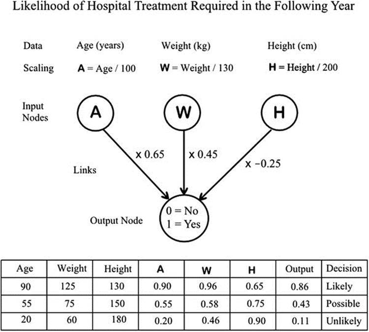
Figure 23-2. A simple neural network illustrating the principle

There may be a layer of nodes between the input nodes and the output node, and these are referred to as hidden nodes. There is an input node for each variable, and the input data is usually scaled to give a value between 0 and 1. The link to the next node will perform a multiplication on this value before passing it on. The multiplication is effectively a weighting factor. The next node will be accepting several values from other input nodes. The added values will then be passed to the output node. The number of nodes to be used has to be decided at the outset, and the number of links may number tens of thousands. The output data are numerical and must be converted back to the required variable values or levels.

The records from the training data are fed in one at a time, and the output is compared with the required value. The error leads to modifications in the link weights, large errors producing large changes and small errors producing small changes. As the process continues, the link weights are revised and the system approaches acceptable outputs short of overfitting. For overfitting can present problems, particularly as it is difficult to see how the processing has taken place. Indeed, there is no logical approach to the process that one could describe, other than that the arithmetic contrives to get the right answers. Because of the complexity in understanding the processing and the required conversion of the output, there have been moves to package neural network programs to suit specific applications.

The simple arrangement of Figure 23-2 has just three input nodes accepting the age, weight, and height of a subject we wish to assess for the possibility of hospital treatment being required in the following year. Each of the input variables (within reasonable limits) is scaled to give a value between 0 and 1. The output is 0 for no and 1 for yes. A set of possible link-weighting values is shown. The outputs for three example sets of input data can be seen to lie between 0 and 1 and may be interpreted as the probability of hospital treatment being required.

Ensembles

With a choice of many different methods and models to use, it is difficult to know at the outset which is likely to be the best for a given set of data. However, it has been found that combining two or more different models can give better predictions than any of the individual models. In effect, a voting procedure is taking place.

These combined models are referred to as ensembles. A remarkable finding with regard to ensembles is that that they do not appear to suffer from overlearning (Siegel, 2013: 148-149). Overlearning, or overfitting as I have described it previously, arises when the analysis has become sophisticated to the point where it is describing the data so fully that the results are sensitive to the detailed features of the data. Siegel likens this advantageous property of ensembles to the behavior of crowds. A group of people guessing, and averaging the result, will usually get closer to the right answer than most of the individuals. Watson, the IBM computer that beat two expert contestants on the US television quiz show Jeopardy! in 2011, was programmed with an ensemble of hundreds of models.

MANHOLE CONTROL

New York City has more than 94,000 miles of underground electrical cables. Manholes provide access to the cables, and periodic faults cause manhole fires, explosions, and smoking manholes. There is an enormous amount of data relating to past events and inspections dating back to the 1880s. The records have been collected and stored by Consolidated Edison, the power utility serving New York City.

In order to radically update the company’s inspection and repair programs, it was decided that the past records could be used to identify the manholes most at risk of a serious incident and those least at risk. This would improve the reliability of the system and public safety.

A team consisting of scientists from Columbia University and engineers from Consolidated Edison took on the task of processing the available data. The raw data was very varied, in that it included records of past events, engineers' records of dealing with events, inspection records, manhole locations, and cable data. Because of the length of time over which information had been collected, there was no consistency in the manner of recording or even in the identification of locations and components.

The raw data was processed to provide an accurate event history over a ten year period for each manhole and a potential 120-year cable history. Combined with inspection results, the data was processed by machine learning algorithms to produce a predictive model aimed at predicting failures of individual manholes.

The model was tested using training data. Data from three boroughs were used: Manhattan, Brooklyn, and the Bronx. Predictions for 2009 were obtained from earlier data and compared with the actual manhole explosions and manhole fires. The top 10% of manholes predicted to have a serious event contained 44% of the ones that did have a serious event, and the top 20% contained 55% of the ones that had a serious event.

The exercise was seen to be of great value in providing a better procedure for electrical grid inspection and repair that could improve public safety and energy reliability. The project demonstrated the value of using all available data, no matter how mixed and confused—big data, not just a selection. The project also demonstrated the value of collecting data for future prediction and not simply as historical records.

_____________________

¹PRISM is an acronym for “PRogramming In Statistical Modeling” (http://sato-www.cs.titech.ac.jp/prism/)—no relation to the United States National Security Agency’s Internet server surveillance program.