Elasticsearch: The Definitive Guide (2015)
Part II. Search in Depth
Chapter 17. Controlling Relevance
Databases that deal purely in structured data (such as dates, numbers, and string enums) have it easy: they just have to check whether a document (or a row, in a relational database) matches the query.
While Boolean yes/no matches are an essential part of full-text search, they are not enough by themselves. Instead, we also need to know how relevant each document is to the query. Full-text search engines have to not only find the matching documents, but also sort them by relevance.
Full-text relevance formulae, or similarity algorithms, combine several factors to produce a single relevance _score for each document. In this chapter, we examine the various moving parts and discuss how they can be controlled.
Of course, relevance is not just about full-text queries; it may need to take structured data into account as well. Perhaps we are looking for a vacation home with particular features (air-conditioning, sea view, free WiFi). The more features that a property has, the more relevant it is. Or perhaps we want to factor in sliding scales like recency, price, popularity, or distance, while still taking the relevance of a full-text query into account.
All of this is possible thanks to the powerful scoring infrastructure available in Elasticsearch.
We will start by looking at the theoretical side of how Lucene calculates relevance, and then move on to practical examples of how you can control the process.
Theory Behind Relevance Scoring
Lucene (and thus Elasticsearch) uses the Boolean model to find matching documents, and a formula called the practical scoring function to calculate relevance. This formula borrows concepts from term frequency/inverse document frequency and the vector space model but adds more-modern features like a coordination factor, field length normalization, and term or query clause boosting.
NOTE
Don’t be alarmed! These concepts are not as complicated as the names make them appear. While this section mentions algorithms, formulae, and mathematical models, it is intended for consumption by mere humans. Understanding the algorithms themselves is not as important as understanding the factors that influence the outcome.
Boolean Model
The Boolean model simply applies the AND, OR, and NOT conditions expressed in the query to find all the documents that match. A query for
full AND text AND search AND (elasticsearch OR lucene)
will include only documents that contain all of the terms full, text, and search, and either elasticsearch or lucene.
This process is simple and fast. It is used to exclude any documents that cannot possibly match the query.
Term Frequency/Inverse Document Frequency (TF/IDF)
Once we have a list of matching documents, they need to be ranked by relevance. Not all documents will contain all the terms, and some terms are more important than others. The relevance score of the whole document depends (in part) on the weight of each query term that appears in that document.
The weight of a term is determined by three factors, which we already introduced in “What Is Relevance?”. The formulae are included for interest’s sake, but you are not required to remember them.
Term frequency
How often does the term appear in this document? The more often, the higher the weight. A field containing five mentions of the same term is more likely to be relevant than a field containing just one mention. The term frequency is calculated as follows:
tf(t in d) = √frequency ![]()
![]()
The term frequency (tf) for term t in document d is the square root of the number of times the term appears in the document.
If you don’t care about how often a term appears in a field, and all you care about is that the term is present, then you can disable term frequencies in the field mapping:
PUT /my_index
{
"mappings": {
"doc": {
"properties": {
"text": {
"type": "string",
"index_options": "docs" ![]()
}
}
}
}
}
![]()
Setting index_options to docs will disable term frequencies and term positions. A field with this mapping will not count how many times a term appears, and will not be usable for phrase or proximity queries. Exact-value not_analyzed string fields use this setting by default.
Inverse document frequency
How often does the term appear in all documents in the collection? The more often, the lower the weight. Common terms like and or the contribute little to relevance, as they appear in most documents, while uncommon terms like elastic or hippopotamus help us zoom in on the most interesting documents. The inverse document frequency is calculated as follows:
idf(t) = 1 + log ( numDocs / (docFreq + 1)) ![]()
![]()
The inverse document frequency (idf) of term t is the logarithm of the number of documents in the index, divided by the number of documents that contain the term.
Field-length norm
How long is the field? The shorter the field, the higher the weight. If a term appears in a short field, such as a title field, it is more likely that the content of that field is about the term than if the same term appears in a much bigger body field. The field length norm is calculated as follows:
norm(d) = 1 / √numTerms ![]()
![]()
The field-length norm (norm) is the inverse square root of the number of terms in the field.
While the field-length norm is important for full-text search, many other fields don’t need norms. Norms consume approximately 1 byte per string field per document in the index, whether or not a document contains the field. Exact-value not_analyzed string fields have norms disabled by default, but you can use the field mapping to disable norms on analyzed fields as well:
PUT /my_index
{
"mappings": {
"doc": {
"properties": {
"text": {
"type": "string",
"norms": { "enabled": false } ![]()
}
}
}
}
}
![]()
This field will not take the field-length norm into account. A long field and a short field will be scored as if they were the same length.
For use cases such as logging, norms are not useful. All you care about is whether a field contains a particular error code or a particular browser identifier. The length of the field does not affect the outcome. Disabling norms can save a significant amount of memory.
Putting it together
These three factors—term frequency, inverse document frequency, and field-length norm—are calculated and stored at index time. Together, they are used to calculate the weight of a single term in a particular document.
TIP
When we refer to documents in the preceding formulae, we are actually talking about a field within a document. Each field has its own inverted index and thus, for TF/IDF purposes, the value of the field is the value of the document.
When we run a simple term query with explain set to true (see “Understanding the Score”), you will see that the only factors involved in calculating the score are the ones explained in the preceding sections:
PUT /my_index/doc/1
{ "text" : "quick brown fox" }
GET /my_index/doc/_search?explain
{
"query": {
"term": {
"text": "fox"
}
}
}
The (abbreviated) explanation from the preceding request is as follows:
weight(text:fox in 0) [PerFieldSimilarity]: 0.15342641 ![]()
result of:
fieldWeight in 0 0.15342641
product of:
tf(freq=1.0), with freq of 1: 1.0 ![]()
idf(docFreq=1, maxDocs=1): 0.30685282 ![]()
fieldNorm(doc=0): 0.5 ![]()
![]()
The final score for term fox in field text in the document with internal Lucene doc ID 0.
![]()
The term fox appears once in the text field in this document.
![]()
The inverse document frequency of fox in the text field in all documents in this index.
![]()
The field-length normalization factor for this field.
Of course, queries usually consist of more than one term, so we need a way of combining the weights of multiple terms. For this, we turn to the vector space model.
Vector Space Model
The vector space model provides a way of comparing a multiterm query against a document. The output is a single score that represents how well the document matches the query. In order to do this, the model represents both the document and the query as vectors.
A vector is really just a one-dimensional array containing numbers, for example:
[1,2,5,22,3,8]
In the vector space model, each number in the vector is the weight of a term, as calculated with term frequency/inverse document frequency.
TIP
While TF/IDF is the default way of calculating term weights for the vector space model, it is not the only way. Other models like Okapi-BM25 exist and are available in Elasticsearch. TF/IDF is the default because it is a simple, efficient algorithm that produces high-quality search results and has stood the test of time.
Imagine that we have a query for “happy hippopotamus.” A common word like happy will have a low weight, while an uncommon term like hippopotamus will have a high weight. Let’s assume that happy has a weight of 2 and hippopotamus has a weight of 5. We can plot this simple two-dimensional vector—[2,5]—as a line on a graph starting at point (0,0) and ending at point (2,5), as shown in Figure 17-1.
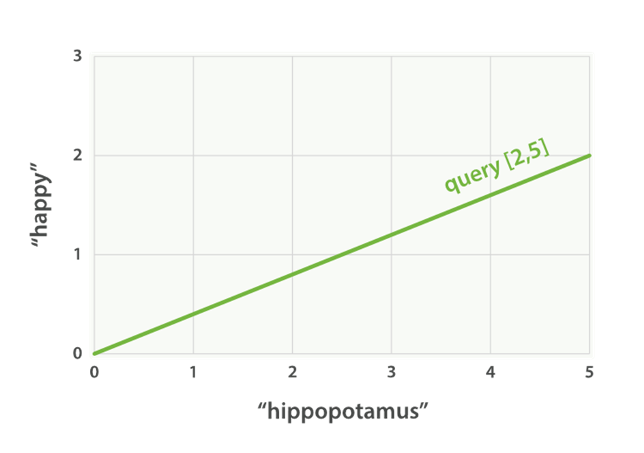
Figure 17-1. A two-dimensional query vector for “happy hippopotamus” represented
Now, imagine we have three documents:
1. I am happy in summer.
2. After Christmas I’m a hippopotamus.
3. The happy hippopotamus helped Harry.
We can create a similar vector for each document, consisting of the weight of each query term—happy and hippopotamus—that appears in the document, and plot these vectors on the same graph, as shown in Figure 17-2:
§ Document 1: (happy,____________)—[2,0]
§ Document 2: ( ___ ,hippopotamus)—[0,5]
§ Document 3: (happy,hippopotamus)—[2,5]
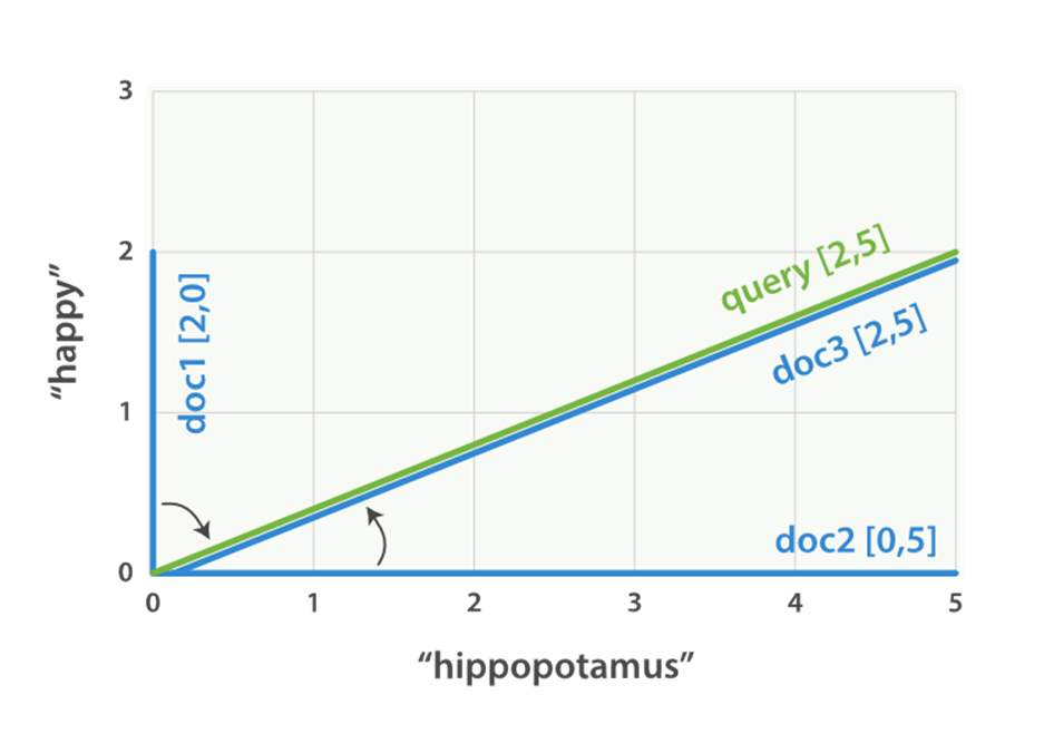
Figure 17-2. Query and document vectors for “happy hippopotamus”
The nice thing about vectors is that they can be compared. By measuring the angle between the query vector and the document vector, it is possible to assign a relevance score to each document. The angle between document 1 and the query is large, so it is of low relevance. Document 2 is closer to the query, meaning that it is reasonably relevant, and document 3 is a perfect match.
TIP
In practice, only two-dimensional vectors (queries with two terms) can be plotted easily on a graph. Fortunately, linear algebra—the branch of mathematics that deals with vectors—provides tools to compare the angle between multidimensional vectors, which means that we can apply the same principles explained above to queries that consist of many terms.
You can read more about how to compare two vectors by using cosine similarity.
Now that we have talked about the theoretical basis of scoring, we can move on to see how scoring is implemented in Lucene.
Lucene’s Practical Scoring Function
For multiterm queries, Lucene takes the Boolean model, TF/IDF, and the vector space model and combines them in a single efficient package that collects matching documents and scores them as it goes.
A multiterm query like
GET /my_index/doc/_search
{
"query": {
"match": {
"text": "quick fox"
}
}
}
is rewritten internally to look like this:
GET /my_index/doc/_search
{
"query": {
"bool": {
"should": [
{"term": { "text": "quick" }},
{"term": { "text": "fox" }}
]
}
}
}
The bool query implements the Boolean model and, in this example, will include only documents that contain either the term quick or the term fox or both.
As soon as a document matches a query, Lucene calculates its score for that query, combining the scores of each matching term. The formula used for scoring is called the practical scoring function. It looks intimidating, but don’t be put off—most of the components you already know. It introduces a few new elements that we discuss next.
score(q,d) = ![]()
queryNorm(q) ![]()
· coord(q,d) ![]()
· ∑ ( ![]()
tf(t in d) ![]()
· idf(t)² ![]()
· t.getBoost() ![]()
· norm(t,d) ![]()
) (t in q) ![]()
![]()
score(q,d) is the relevance score of document d for query q.
![]()
queryNorm(q) is the query normalization factor (new).
![]()
coord(q,d) is the coordination factor (new).
![]()
The sum of the weights for each term t in the query q for document d.
![]()
tf(t in d) is the term frequency for term t in document d.
![]()
idf(t) is the inverse document frequency for term t.
![]()
t.getBoost() is the boost that has been applied to the query (new).
![]()
norm(t,d) is the field-length norm, combined with the index-time field-level boost, if any. (new).
You should recognize score, tf, and idf. The queryNorm, coord, t.getBoost, and norm are new.
We will talk more about query-time boosting later in this chapter, but first let’s get query normalization, coordination, and index-time field-level boosting out of the way.
Query Normalization Factor
The query normalization factor (queryNorm) is an attempt to normalize a query so that the results from one query may be compared with the results of another.
TIP
Even though the intent of the query norm is to make results from different queries comparable, it doesn’t work very well. The only purpose of the relevance _score is to sort the results of the current query in the correct order. You should not try to compare the relevance scores from different queries.
This factor is calculated at the beginning of the query. The actual calculation depends on the queries involved, but a typical implementation is as follows:
queryNorm = 1 / √sumOfSquaredWeights ![]()
![]()
The sumOfSquaredWeights is calculated by adding together the IDF of each term in the query, squared.
TIP
The same query normalization factor is applied to every document, and you have no way of changing it. For all intents and purposes, it can be ignored.
Query Coordination
The coordination factor (coord) is used to reward documents that contain a higher percentage of the query terms. The more query terms that appear in the document, the greater the chances that the document is a good match for the query.
Imagine that we have a query for quick brown fox, and that the weight for each term is 1.5. Without the coordination factor, the score would just be the sum of the weights of the terms in a document. For instance:
§ Document with fox → score: 1.5
§ Document with quick fox → score: 3.0
§ Document with quick brown fox → score: 4.5
The coordination factor multiplies the score by the number of matching terms in the document, and divides it by the total number of terms in the query. With the coordination factor, the scores would be as follows:
§ Document with fox → score: 1.5 * 1 / 3 = 0.5
§ Document with quick fox → score: 3.0 * 2 / 3 = 2.0
§ Document with quick brown fox → score: 4.5 * 3 / 3 = 4.5
The coordination factor results in the document that contains all three terms being much more relevant than the document that contains just two of them.
Remember that the query for quick brown fox is rewritten into a bool query like this:
GET /_search
{
"query": {
"bool": {
"should": [
{ "term": { "text": "quick" }},
{ "term": { "text": "brown" }},
{ "term": { "text": "fox" }}
]
}
}
}
The bool query uses query coordination by default for all should clauses, but it does allow you to disable coordination. Why might you want to do this? Well, usually the answer is, you don’t. Query coordination is usually a good thing. When you use a bool query to wrap several high-level queries like the match query, it also makes sense to leave coordination enabled. The more clauses that match, the higher the degree of overlap between your search request and the documents that are returned.
However, in some advanced use cases, it might make sense to disable coordination. Imagine that you are looking for the synonyms jump, leap, and hop. You don’t care how many of these synonyms are present, as they all represent the same concept. In fact, only one of the synonyms is likely to be present. This would be a good case for disabling the coordination factor:
GET /_search
{
"query": {
"bool": {
"disable_coord": true,
"should": [
{ "term": { "text": "jump" }},
{ "term": { "text": "hop" }},
{ "term": { "text": "leap" }}
]
}
}
}
When you use synonyms (see Chapter 23), this is exactly what happens internally: the rewritten query disables coordination for the synonyms. Most use cases for disabling coordination are handled automatically; you don’t need to worry about it.
Index-Time Field-Level Boosting
We will talk about boosting a field—making it more important than other fields—at query time in “Query-Time Boosting”. It is also possible to apply a boost to a field at index time. Actually, this boost is applied to every term in the field, rather than to the field itself.
To store this boost value in the index without using more space than necessary, this field-level index-time boost is combined with the field-length norm (see “Field-length norm”) and stored in the index as a single byte. This is the value returned by norm(t,d) in the preceding formula.
WARNING
We strongly recommend against using field-level index-time boosts for a few reasons:
§ Combining the boost with the field-length norm and storing it in a single byte means that the field-length norm loses precision. The result is that Elasticsearch is unable to distinguish between a field containing three words and a field containing five words.
§ To change an index-time boost, you have to reindex all your documents. A query-time boost, on the other hand, can be changed with every query.
§ If a field with an index-time boost has multiple values, the boost is multiplied by itself for every value, dramatically increasing the weight for that field.
Query-time boosting is a much simpler, cleaner, more flexible option.
With query normalization, coordination, and index-time boosting out of the way, we can now move on to the most useful tool for influencing the relevance calculation: query-time boosting.
Query-Time Boosting
In Prioritizing Clauses, we explained how you could use the boost parameter at search time to give one query clause more importance than another. For instance:
GET /_search
{
"query": {
"bool": {
"should": [
{
"match": {
"title": {
"query": "quick brown fox",
"boost": 2 ![]()
}
}
},
{
"match": { ![]()
"content": "quick brown fox"
}
}
]
}
}
}
![]()
The title query clause is twice as important as the content query clause, because it has been boosted by a factor of 2.
![]()
A query clause without a boost value has a neutral boost of 1.
Query-time boosting is the main tool that you can use to tune relevance. Any type of query accepts a boost parameter. Setting a boost of 2 doesn’t simply double the final _score; the actual boost value that is applied goes through normalization and some internal optimization. However, it does imply that a clause with a boost of 2 is twice as important as a clause with a boost of 1.
Practically, there is no simple formula for deciding on the “correct” boost value for a particular query clause. It’s a matter of try-it-and-see. Remember that boost is just one of the factors involved in the relevance score; it has to compete with the other factors. For instance, in the preceding example, the title field will probably already have a “natural” boost over the content field thanks to the field-length norm (titles are usually shorter than the related content), so don’t blindly boost fields just because you think they should be boosted. Apply a boost and check the results. Change the boost and check again.
Boosting an Index
When searching across multiple indices, you can boost an entire index over the others with the indices_boost parameter. This could be used, as in the next example, to give more weight to documents from a more recent index:
GET /docs_2014_*/_search ![]()
{
"indices_boost": { ![]()
"docs_2014_10": 3,
"docs_2014_09": 2
},
"query": {
"match": {
"text": "quick brown fox"
}
}
}
![]()
This multi-index search covers all indices beginning with docs_2014_.
![]()
Documents in the docs_2014_10 index will be boosted by 3, those in docs_2014_09 by 2, and any other matching indices will have a neutral boost of 1.
t.getBoost()
These boost values are represented in the “Lucene’s Practical Scoring Function” by the t.getBoost() element. Boosts are not applied at the level that they appear in the query DSL. Instead, any boost values are combined and passsed down to the individual terms. The t.getBoost()method returns any boost value applied to the term itself or to any of the queries higher up the chain.
TIP
In fact, reading the explain output is a little more complex than that. You won’t see the boost value or t.getBoost() mentioned in the explanation at all. Instead, the boost is rolled into the queryNorm that is applied to a particular term. Although we said that the queryNorm is the same for every term, you will see that the queryNorm for a boosted term is higher than the queryNorm for an unboosted term.
Manipulating Relevance with Query Structure
The Elasticsearch query DSL is immensely flexible. You can move individual query clauses up and down the query hierarchy to make a clause more or less important. For instance, imagine the following query:
quick OR brown OR red OR fox
We could write this as a bool query with all terms at the same level:
GET /_search
{
"query": {
"bool": {
"should": [
{ "term": { "text": "quick" }},
{ "term": { "text": "brown" }},
{ "term": { "text": "red" }},
{ "term": { "text": "fox" }}
]
}
}
}
But this query might score a document that contains quick, red, and brown the same as another document that contains quick, red, and fox. Red and brown are synonyms and we probably only need one of them to match. Perhaps we really want to express the query as follows:
quick OR (brown OR red) OR fox
According to standard Boolean logic, this is exactly the same as the original query, but as we have already seen in Combining Queries, a bool query does not concern itself only with whether a document matches, but also with how well it matches.
A better way to write this query is as follows:
GET /_search
{
"query": {
"bool": {
"should": [
{ "term": { "text": "quick" }},
{ "term": { "text": "fox" }},
{
"bool": {
"should": [
{ "term": { "text": "brown" }},
{ "term": { "text": "red" }}
]
}
}
]
}
}
}
Now, red and brown compete with each other at their own level, and quick, fox, and red OR brown are the top-level competitive terms.
We have already discussed how the match, multi_match, term, bool, and dis_max queries can be used to manipulate scoring. In the rest of this chapter, we present three other scoring-related queries: the boosting query, the constant_score query, and the function_score query.
Not Quite Not
A search on the Internet for “Apple” is likely to return results about the company, the fruit, and various recipes. We could try to narrow it down to just the company by excluding words like pie, tart, crumble, and tree, using a must_not clause in a bool query:
GET /_search
{
"query": {
"bool": {
"must": {
"match": {
"text": "apple"
}
},
"must_not": {
"match": {
"text": "pie tart fruit crumble tree"
}
}
}
}
}
But who is to say that we wouldn’t miss a very relevant document about Apple the company by excluding tree or crumble? Sometimes, must_not can be too strict.
boosting Query
The boosting query solves this problem. It allows us to still include results that appear to be about the fruit or the pastries, but to downgrade them—to rank them lower than they would otherwise be:
GET /_search
{
"query": {
"boosting": {
"positive": {
"match": {
"text": "apple"
}
},
"negative": {
"match": {
"text": "pie tart fruit crumble tree"
}
},
"negative_boost": 0.5
}
}
}
It accepts a positive query and a negative query. Only documents that match the positive query will be included in the results list, but documents that also match the negative query will be downgraded by multiplying the original _score of the document with thenegative_boost.
For this to work, the negative_boost must be less than 1.0. In this example, any documents that contain any of the negative terms will have their _score cut in half.
Ignoring TF/IDF
Sometimes we just don’t care about TF/IDF. All we want to know is that a certain word appears in a field. Perhaps we are searching for a vacation home and we want to find houses that have as many of these features as possible:
§ WiFi
§ Garden
§ Pool
The vacation home documents look something like this:
{ "description": "A delightful four-bedroomed house with ... " }
We could use a simple match query:
GET /_search
{
"query": {
"match": {
"description": "wifi garden pool"
}
}
}
However, this isn’t really full-text search. In this case, TF/IDF just gets in the way. We don’t care whether wifi is a common term, or how often it appears in the document. All we care about is that it does appear. In fact, we just want to rank houses by the number of features they have—the more, the better. If a feature is present, it should score 1, and if it isn’t, 0.
constant_score Query
Enter the constant_score query. This query can wrap either a query or a filter, and assigns a score of 1 to any documents that match, regardless of TF/IDF:
GET /_search
{
"query": {
"bool": {
"should": [
{ "constant_score": {
"query": { "match": { "description": "wifi" }}
}},
{ "constant_score": {
"query": { "match": { "description": "garden" }}
}},
{ "constant_score": {
"query": { "match": { "description": "pool" }}
}}
]
}
}
}
Perhaps not all features are equally important—some have more value to the user than others. If the most important feature is the pool, we could boost that clause to make it count for more:
GET /_search
{
"query": {
"bool": {
"should": [
{ "constant_score": {
"query": { "match": { "description": "wifi" }}
}},
{ "constant_score": {
"query": { "match": { "description": "garden" }}
}},
{ "constant_score": {
"boost": 2 ![]()
"query": { "match": { "description": "pool" }}
}}
]
}
}
}
![]()
A matching pool clause would add a score of 2, while the other clauses would add a score of only 1 each.
NOTE
The final score for each result is not simply the sum of the scores of all matching clauses. The coordination factor and query normalization factor are still taken into account.
We could improve our vacation home documents by adding a not_analyzed features field to our vacation homes:
{ "features": [ "wifi", "pool", "garden" ] }
By default, a not_analyzed field has field-length norms disabled and has index_options set to docs, disabling term frequencies, but the problem remains: the inverse document frequency of each term is still taken into account.
We could use the same approach that we used previously, with the constant_score query:
GET /_search
{
"query": {
"bool": {
"should": [
{ "constant_score": {
"query": { "match": { "features": "wifi" }}
}},
{ "constant_score": {
"query": { "match": { "features": "garden" }}
}},
{ "constant_score": {
"boost": 2
"query": { "match": { "features": "pool" }}
}}
]
}
}
}
Really, though, each of these features should be treated like a filter. A vacation home either has the feature or it doesn’t—a filter seems like it would be a natural fit. On top of that, if we use filters, we can benefit from filter caching.
The problem is this: filters don’t score. What we need is a way of bridging the gap between filters and queries. The function_score query does this and a whole lot more.
function_score Query
The function_score query is the ultimate tool for taking control of the scoring process. It allows you to apply a function to each document that matches the main query in order to alter or completely replace the original query _score.
In fact, you can apply different functions to subsets of the main result set by using filters, which gives you the best of both worlds: efficient scoring with cacheable filters.
It supports several predefined functions out of the box:
weight
Apply a simple boost to each document without the boost being normalized: a weight of 2 results in 2 * _score.
field_value_factor
Use the value of a field in the document to alter the _score, such as factoring in a popularity count or number of votes.
random_score
Use consistently random scoring to sort results differently for every user, while maintaining the same sort order for a single user.
Decay functions—linear, exp, gauss
Incorporate sliding-scale values like publish_date, geo_location, or price into the _score to prefer recently published documents, documents near a latitude/longitude (lat/lon) point, or documents near a specified price point.
script_score
Use a custom script to take complete control of the scoring logic. If your needs extend beyond those of the functions in this list, write a custom script to implement the logic that you need.
Without the function_score query, we would not be able to combine the score from a full-text query with a factor like recency. We would have to sort either by _score or by date; the effect of one would obliterate the effect of the other. This query allows you to blend the two together: to still sort by full-text relevance, but giving extra weight to recently published documents, or popular documents, or products that are near the user’s price point. As you can imagine, a query that supports all of this can look fairly complex. We’ll start with a simple use case and work our way up the complexity ladder.
Boosting by Popularity
Imagine that we have a website that hosts blog posts and enables users to vote for the blog posts that they like. We would like more-popular posts to appear higher in the results list, but still have the full-text score as the main relevance driver. We can do this easily by storing the number of votes with each blog post:
PUT /blogposts/post/1
{
"title": "About popularity",
"content": "In this post we will talk about...",
"votes": 6
}
At search time, we can use the function_score query with the field_value_factor function to combine the number of votes with the full-text relevance score:
GET /blogposts/post/_search
{
"query": {
"function_score": { ![]()
"query": { ![]()
"multi_match": {
"query": "popularity",
"fields": [ "title", "content" ]
}
},
"field_value_factor": { ![]()
"field": "votes" ![]()
}
}
}
}
![]()
The function_score query wraps the main query and the function we would like to apply.
![]()
The main query is executed first.
![]()
The field_value_factor function is applied to every document matching the main query.
![]()
Every document must have a number in the votes field for the function_score to work.
In the preceding example, the final _score for each document has been altered as follows:
new_score = old_score * number_of_votes
This will not give us great results. The full-text _score range usually falls somewhere between 0 and 10. As can be seen in Figure 17-3, a blog post with 10 votes will completely swamp the effect of the full-text score, and a blog post with 0 votes will reset the score to zero.
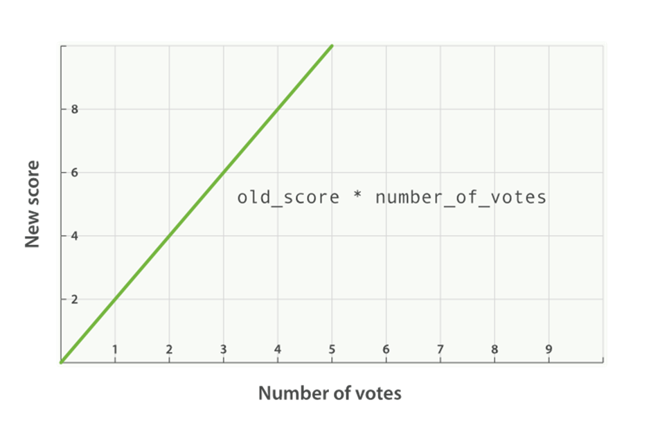
Figure 17-3. Linear popularity based on an original _score of 2.0
modifier
A better way to incorporate popularity is to smooth out the votes value with some modifier. In other words, we want the first few votes to count a lot, but for each subsequent vote to count less. The difference between 0 votes and 1 vote should be much bigger than the difference between 10 votes and 11 votes.
A typical modifier for this use case is log1p, which changes the formula to the following:
new_score = old_score * log(1 + number_of_votes)
The log function smooths out the effect of the votes field to provide a curve like the one in Figure 17-4.
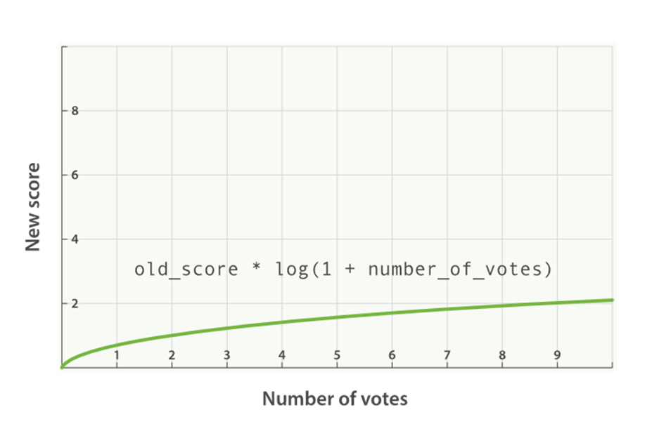
Figure 17-4. Logarithmic popularity based on an original _score of 2.0
The request with the modifier parameter looks like the following:
GET /blogposts/post/_search
{
"query": {
"function_score": {
"query": {
"multi_match": {
"query": "popularity",
"fields": [ "title", "content" ]
}
},
"field_value_factor": {
"field": "votes",
"modifier": "log1p" ![]()
}
}
}
}
![]()
Set the modifier to log1p.
The available modifiers are none (the default), log, log1p, log2p, ln, ln1p, ln2p, square, sqrt, and reciprocal. You can read more about them in the field_value_factor documentation.
factor
The strength of the popularity effect can be increased or decreased by multiplying the value in the votes field by some number, called the factor:
GET /blogposts/post/_search
{
"query": {
"function_score": {
"query": {
"multi_match": {
"query": "popularity",
"fields": [ "title", "content" ]
}
},
"field_value_factor": {
"field": "votes",
"modifier": "log1p",
"factor": 2 ![]()
}
}
}
}
![]()
Doubles the popularity effect
Adding in a factor changes the formula to this:
new_score = old_score * log(1 + factor * number_of_votes)
A factor greater than 1 increases the effect, and a factor less than 1 decreases the effect, as shown in Figure 17-5.
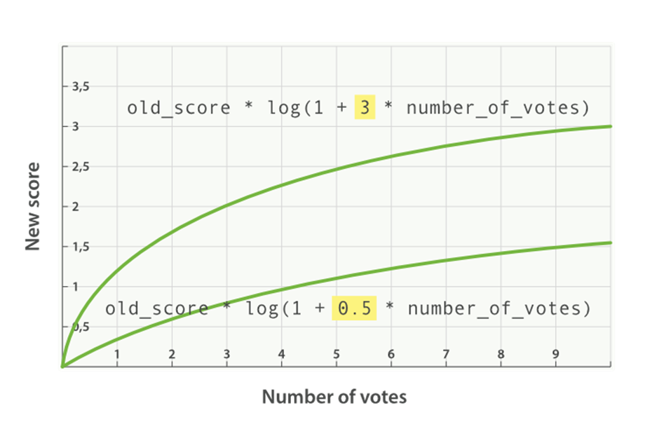
Figure 17-5. Logarithmic popularity with different factors
boost_mode
Perhaps multiplying the full-text score by the result of the field_value_factor function still has too large an effect. We can control how the result of a function is combined with the _score from the query by using the boost_mode parameter, which accepts the following values:
multiply
Multiply the _score with the function result (default)
sum
Add the function result to the _score
min
The lower of the _score and the function result
max
The higher of the _score and the function result
replace
Replace the _score with the function result
If, instead of multiplying, we add the function result to the _score, we can achieve a much smaller effect, especially if we use a low factor:
GET /blogposts/post/_search
{
"query": {
"function_score": {
"query": {
"multi_match": {
"query": "popularity",
"fields": [ "title", "content" ]
}
},
"field_value_factor": {
"field": "votes",
"modifier": "log1p",
"factor": 0.1
},
"boost_mode": "sum" ![]()
}
}
}
![]()
Add the function result to the _score.
The formula for the preceding request now looks like this (see Figure 17-6):
new_score = old_score + log(1 + 0.1 * number_of_votes)
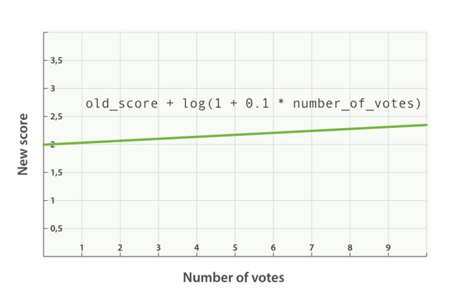
Figure 17-6. Combining popularity with sum
max_boost
Finally, we can cap the maximum effect that the function can have by using the max_boost parameter:
GET /blogposts/post/_search
{
"query": {
"function_score": {
"query": {
"multi_match": {
"query": "popularity",
"fields": [ "title", "content" ]
}
},
"field_value_factor": {
"field": "votes",
"modifier": "log1p",
"factor": 0.1
},
"boost_mode": "sum",
"max_boost": 1.5 ![]()
}
}
}
![]()
Whatever the result of the field_value_factor function, it will never be greater than 1.5.
NOTE
The max_boost applies a limit to the result of the function only, not to the final _score.
Boosting Filtered Subsets
Let’s return to the problem that we were dealing with in “Ignoring TF/IDF”, where we wanted to score vacation homes by the number of features that each home possesses. We ended that section by wishing for a way to use cached filters to affect the score, and with the function_scorequery we can do just that.
The examples we have shown thus far have used a single function for all documents. Now we want to divide the results into subsets by using filters (one filter per feature), and apply a different function to each subset.
The function that we will use in this example is the weight, which is similar to the boost parameter accepted by any query. The difference is that the weight is not normalized by Lucene into some obscure floating-point number; it is used as is.
The structure of the query has to change somewhat to incorporate multiple functions:
GET /_search
{
"query": {
"function_score": {
"filter": { ![]()
"term": { "city": "Barcelona" }
},
"functions": [ ![]()
{
"filter": { "term": { "features": "wifi" }}, ![]()
"weight": 1
},
{
"filter": { "term": { "features": "garden" }}, ![]()
"weight": 1
},
{
"filter": { "term": { "features": "pool" }}, ![]()
"weight": 2 ![]()
}
],
"score_mode": "sum", ![]()
}
}
}
![]()
This function_score query has a filter instead of a query.
![]()
The functions key holds a list of functions that should be applied.
![]()
The function is applied only if the document matches the (optional) filter.
![]()
The pool feature is more important than the others so it has a higher weight.
![]()
The score_mode specifies how the values from each function should be combined.
The new features to note in this example are explained in the following sections.
filter Versus query
The first thing to note is that we have specified a filter instead of a query. In this example, we do not need full-text search. We just want to return all documents that have Barcelona in the city field, logic that is better expressed as a filter instead of a query. All documents returned by the filter will have a _score of 1. The function_score query accepts either a query or a filter. If neither is specified, it will default to using the match_all query.
functions
The functions key holds an array of functions to apply. Each entry in the array may also optionally specify a filter, in which case the function will be applied only to documents that match that filter. In this example, we apply a weight of 1 (or 2 in the case of pool) to any document that matches the filter.
score_mode
Each function returns a result, and we need a way of reducing these multiple results to a single value that can be combined with the original _score. This is the role of the score_mode parameter, which accepts the following values:
multiply
Function results are multiplied together (default).
sum
Function results are added up.
avg
The average of all the function results.
max
The highest function result is used.
min
The lowest function result is used.
first
Uses only the result from the first function that either doesn’t have a filter or that has a filter matching the document.
In this case, we want to add the weight results from each matching filter together to produce the final score, so we have used the sum score mode.
Documents that don’t match any of the filters will keep their original _score of 1.
Random Scoring
You may have been wondering what consistently random scoring is, or why you would ever want to use it. The previous example provides a good use case. All results from the previous example would receive a final _score of 1, 2, 3, 4, or 5. Maybe there are only a few homes that score 5, but presumably there would be a lot of homes scoring 2 or 3.
As the owner of the website, you want to give your advertisers as much exposure as possible. With the current query, results with the same _score would be returned in the same order every time. It would be good to introduce some randomness here, to ensure that all documents in a single score level get a similar amount of exposure.
We want every user to see a different random order, but we want the same user to see the same order when clicking on page 2, 3, and so forth. This is what is meant by consistently random.
The random_score function, which outputs a number between 0 and 1, will produce consistently random results when it is provided with the same seed value, such as a user’s session ID:
GET /_search
{
"query": {
"function_score": {
"filter": {
"term": { "city": "Barcelona" }
},
"functions": [
{
"filter": { "term": { "features": "wifi" }},
"weight": 1
},
{
"filter": { "term": { "features": "garden" }},
"weight": 1
},
{
"filter": { "term": { "features": "pool" }},
"weight": 2
},
{
"random_score": { ![]()
"seed": "the users session id" ![]()
}
}
],
"score_mode": "sum",
}
}
}
![]()
The random_score clause doesn’t have any filter, so it will be applied to all documents.
![]()
Pass the user’s session ID as the seed, to make randomization consistent for that user. The same seed will result in the same randomization.
Of course, if you index new documents that match the query, the order of results will change regardless of whether you use consistent randomization or not.
The Closer, The Better
Many variables could influence the user’s choice of vacation home. Maybe she would like to be close to the center of town, but perhaps would be willing to settle for a place that is a bit farther from the center if the price is low enough. Perhaps the reverse is true: she would be willing to pay more for the best location.
If we were to add a filter that excluded any vacation homes farther than 1 kilometer from the center, or any vacation homes that cost more than £100 a night, we might exclude results that the user would consider to be a good compromise.
The function_score query gives us the ability to trade off one sliding scale (like location) against another sliding scale (like price), with a group of functions known as the decay functions.
The three decay functions—called linear, exp, and gauss—operate on numeric fields, date fields, or lat/lon geo-points. All three take the same parameters:
origin
The central point, or the best possible value for the field. Documents that fall at the origin will get a full _score of 1.0.
scale
The rate of decay—how quickly the _score should drop the further from the origin that a document lies (for example, every £10 or every 100 meters).
decay
The _score that a document at scale distance from the origin should receive. Defaults to 0.5.
offset
Setting a nonzero offset expands the central point to cover a range of values instead of just the single point specified by the origin. All values in the range -offset <= origin <= +offset will receive the full _score of 1.0.
The only difference between these three functions is the shape of the decay curve. The difference is most easily illustrated with a graph (see Figure 17-7).
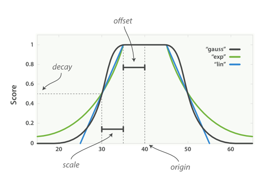
Figure 17-7. Decay function curves
The curves shown in Figure 17-7 all have their origin—the central point—set to 40. The offset is 5, meaning that all values in the range 40 - 5 <= value <= 40 + 5 are treated as though they were at the origin—they all get the full score of 1.0.
Outside this range, the score starts to decay. The rate of decay is determined by the scale (which in this example is set to 5), and the decay (which is set to the default of 0.5). The result is that all three curves return a score of 0.5 at origin +/- (offset + scale), or at points 30 and50.
The difference between linear, exp, and gauss is the shape of the curve at other points in the range:
§ The linear funtion is just a straight line. Once the line hits zero, all values outside the line will return a score of 0.0.
§ The exp (exponential) function decays rapidly, then slows down.
§ The gauss (Gaussian) function is bell-shaped—it decays slowly, then rapidly, then slows down again.
Which curve you choose depends entirely on how quickly you want the _score to decay, the further a value is from the origin.
To return to our example: our user would prefer to rent a vacation home close to the center of London ({ "lat": 51.50, "lon": 0.12}) and to pay no more than £100 a night, but our user considers price to be more important than distance. We could write this query as follows:
GET /_search
{
"query": {
"function_score": {
"functions": [
{
"gauss": {
"location": { ![]()
"origin": { "lat": 51.5, "lon": 0.12 },
"offset": "2km",
"scale": "3km"
}
}
},
{
"gauss": {
"price": { ![]()
"origin": "50", ![]()
"offset": "50",
"scale": "20"
}
},
"weight": 2 ![]()
}
]
}
}
}
![]()
The location field is mapped as a geo_point.
![]()
The price field is numeric.
![]()
See “Understanding the price Clause” for the reason that origin is 50 instead of 100.
![]()
The price clause has twice the weight of the location clause.
The location clause is easy to understand:
§ We have specified an origin that corresponds to the center of London.
§ Any location within 2km of the origin receives the full score of 1.0.
§ Locations 5km (offset + scale) from the centre receive a score of 0.5.
Understanding the price Clause
The price clause is a little trickier. The user’s preferred price is anything up to £100, but this example sets the origin to £50. Prices can’t be negative, but the lower they are, the better. Really, any price between £0 and £100 should be considered optimal.
If we were to set the origin to £100, then prices below £100 would receive a lower score. Instead, we set both the origin and the offset to £50. That way, the score decays only for any prices above £100 (origin + offset).
TIP
The weight parameter can be used to increase or decrease the contribution of individual clauses. The weight, which defaults to 1.0, is multiplied by the score from each clause before the scores are combined with the specified score_mode.
Scoring with Scripts
Finally, if none of the function_score’s built-in functions suffice, you can implement the logic that you need with a script, using the script_score function.
For an example, let’s say that we want to factor our profit margin into the relevance calculation. In our business, the profit margin depends on three factors:
§ The price per night of the vacation home.
§ The user’s membership level—some levels get a percentage discount above a certain price per night threshold.
§ The negotiated margin as a percentage of the price-per-night, after user discounts.
The algorithm that we will use to calculate the profit for each home is as follows:
if (price < threshold) {
profit = price * margin
} else {
profit = price * (1 - discount) * margin;
}
We probably don’t want to use the absolute profit as a score; it would overwhelm the other factors like location, popularity and features. Instead, we can express the profit as a percentage of our target profit. A profit margin above our target will have a positive score (greater than 1.0), and a profit margin below our target will have a negative score (less than 1.0):
if (price < threshold) {
profit = price * margin
} else {
profit = price * (1 - discount) * margin
}
return profit / target
The default scripting language in Elasticsearch is Groovy, which for the most part looks a lot like JavaScript. The preceding algorithm as a Groovy script would look like this:
price = doc['price'].value ![]()
margin = doc['margin'].value ![]()
if (price < threshold) { ![]()
return price * margin / target
}
return price * (1 - discount) * margin / target ![]()
![]()
The price and margin variables are extracted from the price and margin fields in the document.
![]()
The threshold, discount, and target variables we will pass in as params.
Finally, we can add our script_score function to the list of other functions that we are already using:
GET /_search
{
"function_score": {
"functions": [
{ ...location clause... }, ![]()
{ ...price clause... }, ![]()
{
"script_score": {
"params": { ![]()
"threshold": 80,
"discount": 0.1,
"target": 10
},
"script": "price = doc['price'].value; margin = doc['margin'].value;
if (price < threshold) { return price * margin / target };
return price * (1 - discount) * margin / target;" ![]()
}
}
]
}
}
![]()
The location and price clauses refer to the example explained in “The Closer, The Better”.
![]()
By passing in these variables as params, we can change their values every time we run this query without having to recompile the script.
![]()
JSON cannot include embedded newline characters. Newline characters in the script should either be escaped as \n or replaced with semicolons.
This query would return the documents that best satisfy the user’s requirements for location and price, while still factoring in our need to make a profit.
TIP
The script_score function provides enormous flexibility. Within a script, you have access to the fields of the document, to the current _score, and even to the term frequencies, inverse document frequencies, and field length norms (see Text scoring in scripts).
That said, scripts can have a performance impact. If you do find that your scripts are not quite fast enough, you have three options:
§ Try to precalculate as much information as possible and include it in each document.
§ Groovy is fast, but not quite as fast as Java. You could reimplement your script as a native Java script. (See Native Java Scripts).
§ Use the rescore functionality described in “Rescoring Results” to apply your script to only the best-scoring documents.
Pluggable Similarity Algorithms
Before we move on from relevance and scoring, we will finish this chapter with a more advanced subject: pluggable similarity algorithms. While Elasticsearch uses the “Lucene’s Practical Scoring Function” as its default similarity algorithm, it supports other algorithms out of the box, which are listed in the Similarity Modules documentation.
Okapi BM25
The most interesting competitor to TF/IDF and the vector space model is called Okapi BM25, which is considered to be a state-of-the-art ranking function. BM25 originates from the probabilistic relevance model, rather than the vector space model, yet the algorithm has a lot in common with Lucene’s practical scoring function.
Both use of term frequency, inverse document frequency, and field-length normalization, but the definition of each of these factors is a little different. Rather than explaining the BM25 formula in detail, we will focus on the practical advantages that BM25 offers.
Term-frequency saturation
Both TF/IDF and BM25 use inverse document frequency to distinguish between common (low value) words and uncommon (high value) words. Both also recognize (see “Term frequency”) that the more often a word appears in a document, the more likely is it that the document is relevant for that word.
However, common words occur commonly. The fact that a common word appears many times in one document is offset by the fact that the word appears many times in all documents.
However, TF/IDF was designed in an era when it was standard practice to remove the most common words (or stopwords, see Chapter 22) from the index altogether. The algorithm didn’t need to worry about an upper limit for term frequency because the most frequent terms had already been removed.
In Elasticsearch, the standard analyzer—the default for string fields—doesn’t remove stopwords because, even though they are words of little value, they do still have some value. The result is that, for very long documents, the sheer number of occurrences of words like the and andcan artificially boost their weight.
BM25, on the other hand, does have an upper limit. Terms that appear 5 to 10 times in a document have a significantly larger impact on relevance than terms that appear just once or twice. However, as can be seen in Figure 17-8, terms that appear 20 times in a document have almost the same impact as terms that appear a thousand times or more.
This is known as nonlinear term-frequency saturation.
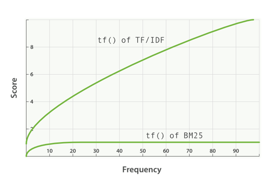
Figure 17-8. Term frequency saturation for TF/IDF and BM25
Field-length normalization
In “Field-length norm”, we said that Lucene considers shorter fields to have more weight than longer fields: the frequency of a term in a field is offset by the length of the field. However, the practical scoring function treats all fields in the same way. It will treat all title fields (because they are short) as more important than all body fields (because they are long).
BM25 also considers shorter fields to have more weight than longer fields, but it considers each field separately by taking the average length of the field into account. It can distinguish between a short title field and a long title field.
Caution
In “Query-Time Boosting”, we said that the title field has a natural boost over the body field because of its length. This natural boost disappears with BM25 as differences in field length apply only within a single field.
Tuning BM25
One of the nice features of BM25 is that, unlike TF/IDF, it has two parameters that allow it to be tuned:
k1
This parameter controls how quickly an increase in term frequency results in term-frequency saturation. The default value is 1.2. Lower values result in quicker saturation, and higher values in slower saturation.
b
This parameter controls how much effect field-length normalization should have. A value of 0.0 disables normalization completely, and a value of 1.0 normalizes fully. The default is 0.75.
The practicalities of tuning BM25 are another matter. The default values for k1 and b should be suitable for most document collections, but the optimal values really depend on the collection. Finding good values for your collection is a matter of adjusting, checking, and adjusting again.
Changing Similarities
The similarity algorithm can be set on a per-field basis. It’s just a matter of specifying the chosen algorithm in the field’s mapping:
PUT /my_index
{
"mappings": {
"doc": {
"properties": {
"title": {
"type": "string",
"similarity": "BM25" ![]()
},
"body": {
"type": "string",
"similarity": "default" ![]()
}
}
}
}
![]()
The title field uses BM25 similarity.
![]()
The body field uses the default similarity (see “Lucene’s Practical Scoring Function”).
Currently, it is not possible to change the similarity mapping for an existing field. You would need to reindex your data in order to do that.
Configuring BM25
Configuring a similarity is much like configuring an analyzer. Custom similarities can be specified when creating an index. For instance:
PUT /my_index
{
"settings": {
"similarity": {
"my_bm25": { ![]()
"type": "BM25",
"b": 0 ![]()
}
}
},
"mappings": {
"doc": {
"properties": {
"title": {
"type": "string",
"similarity": "my_bm25" ![]()
},
"body": {
"type": "string",
"similarity": "BM25" ![]()
}
}
}
}
}
![]()
Create a custom similarity called my_bm25, based on the built-in BM25 similarity.
![]()
Disable field-length normalization. See “Tuning BM25”.
![]()
Field title uses the custom similarity my_bm25.
![]()
Field body uses the built-in similarity BM25.
TIP
A custom similarity can be updated by closing the index, updating the index settings, and reopening the index. This allows you to experiment with different configurations without having to reindex your documents.
Relevance Tuning Is the Last 10%
In this chapter, we looked at a how Lucene generates scores based on TF/IDF. Understanding the score-generation process is critical so you can tune, modulate, attenuate, and manipulate the score for your particular business domain.
In practice, simple combinations of queries will get you good search results. But to get great search results, you’ll often have to start tinkering with the previously mentioned tuning methods.
Often, applying a boost on a strategic field or rearranging a query to emphasize a particular clause will be sufficient to make your results great. Sometimes you’ll need more-invasive changes. This is usually the case if your scoring requirements diverge heavily from Lucene’s word-based TF/IDF model (for example, you want to score based on time or distance).
With that said, relevancy tuning is a rabbit hole that you can easily fall into and never emerge. The concept of most relevant is a nebulous target to hit, and different people often have different ideas about document ranking. It is easy to get into a cycle of constant fiddling without any apparent progress.
We encourage you to avoid this (very tempting) behavior and instead properly instrument your search results. Monitor how often your users click the top result, the top 10, and the first page; how often they execute a secondary query without selecting a result first; how often they click a result and immediately go back to the search results, and so forth.
These are all indicators of how relevant your search results are to the user. If your query is returning highly relevant results, users will select one of the top-five results, find what they want, and leave. Irrelevant results cause users to click around and try new search queries.
Once you have instrumentation in place, tuning your query is simple. Make a change, monitor its effect on your users, and repeat as necessary. The tools outlined in this chapter are just that: tools. You have to use them appropriately to propel your search results into the great category, and the only way to do that is with strong measurement of user behavior.
All materials on the site are licensed Creative Commons Attribution-Sharealike 3.0 Unported CC BY-SA 3.0 & GNU Free Documentation License (GFDL)
If you are the copyright holder of any material contained on our site and intend to remove it, please contact our site administrator for approval.
© 2016-2025 All site design rights belong to S.Y.A.