Elasticsearch: The Definitive Guide (2015)
Part IV. Aggregations
Chapter 28. Looking at Time
If search is the most popular activity in Elasticsearch, building date histograms must be the second most popular. Why would you want to use a date histogram?
Imagine your data has a timestamp. It doesn’t matter what the data is—Apache log events, stock buy/sell transaction dates, baseball game times—anything with a timestamp can benefit from the date histogram. When you have a timestamp, you often want to build metrics that are expressedover time:
§ How many cars sold each month this year?
§ What was the price of this stock for the last 12 hours?
§ What was the average latency of our website every hour in the last week?
While regular histograms are often represented as bar charts, date histograms tend to be converted into line graphs representing time series. Many companies use Elasticsearch solely for analytics over time series data. The date_histogram bucket is their bread and butter.
The date_histogram bucket works similarly to the regular histogram. Rather than building buckets based on a numeric field representing numeric ranges, it builds buckets based on time ranges. Each bucket is therefore defined as a certain calendar size (for example, 1 month or 2.5 days).
CAN A REGULAR HISTOGRAM WORK WITH DATES?
Technically, yes. A regular histogram bucket will work with dates. However, it is not calendar-aware. With the date_histogram, you can specify intervals such as 1 month, which knows that February is shorter than December. The date_histogram also has the advantage of being able to work with time zones, which allows you to customize graphs to the time zone of the user, not the server.
The regular histogram will interpret dates as numbers, which means you must specify intervals in terms of milliseconds. And the aggregation doesn’t know about calendar intervals, which makes it largely useless for dates.
Our first example will build a simple line chart to answer this question: how many cars were sold each month?
GET /cars/transactions/_search?search_type=count
{
"aggs": {
"sales": {
"date_histogram": {
"field": "sold",
"interval": "month", ![]()
"format": "yyyy-MM-dd" ![]()
}
}
}
}
![]()
The interval is requested in calendar terminology (for example, one month per bucket).
![]()
We provide a date format so that bucket keys are pretty.
Our query has a single aggregation, which builds a bucket per month. This will give us the number of cars sold in each month. An additional format parameter is provided so the buckets have “pretty” keys. Internally, dates are simply represented as a numeric value. This tends to make UI designers grumpy, however, so a prettier format can be specified using common date formatting.
The response is both expected and a little surprising (see if you can spot the surprise):
{
...
"aggregations": {
"sales": {
"buckets": [
{
"key_as_string": "2014-01-01",
"key": 1388534400000,
"doc_count": 1
},
{
"key_as_string": "2014-02-01",
"key": 1391212800000,
"doc_count": 1
},
{
"key_as_string": "2014-05-01",
"key": 1398902400000,
"doc_count": 1
},
{
"key_as_string": "2014-07-01",
"key": 1404172800000,
"doc_count": 1
},
{
"key_as_string": "2014-08-01",
"key": 1406851200000,
"doc_count": 1
},
{
"key_as_string": "2014-10-01",
"key": 1412121600000,
"doc_count": 1
},
{
"key_as_string": "2014-11-01",
"key": 1414800000000,
"doc_count": 2
}
]
...
}
The aggregation is represented in full. As you can see, we have buckets that represent months, a count of docs in each month, and our pretty key_as_string.
Returning Empty Buckets
Notice something odd about that last response?
Yep, that’s right. We are missing a few months! By default, the date_histogram (and histogram too) returns only buckets that have a nonzero document count.
This means your histogram will be a minimal response. Often, this is not the behavior you want. For many applications, you would like to dump the response directly into a graphing library without doing any post-processing.
Essentially, we want buckets even if they have a count of zero. We can set two additional parameters that will provide this 'margin-top:0cm;margin-right:0cm;margin-bottom:0cm; margin-left:20.0pt;margin-bottom:.0001pt;line-height:normal;vertical-align: baseline'>GET /cars/transactions/_search?search_type=count
{
"aggs": {
"sales": {
"date_histogram": {
"field":"sold",
"interval": "month",
"format": "yyyy-MM-dd",
"min_doc_count":0, ![]()
"extended_bounds" : { ![]()
"min" :"2014-01-01",
"max" : "2014-12-31"
}
}
}
}
}
![]()
This parameter forces empty buckets to be returned.
![]()
This parameter forces the entire year to be returned.
The two additional parameters will force the response to return all months in the year, regardless of their doc count. The min_doc_count is very understandable: it forces buckets to be returned even if they are empty.
The extended_bounds parameter requires a little explanation. The min_doc_count parameter forces empty buckets to be returned, but by default Elasticsearch will return only buckets that are between the minimum and maximum value in your data.
So if your data falls between April and July, you’ll have buckets representing only those months (empty or otherwise). To get the full year, we need to tell Elasticsearch that we want buckets even if they fall before the minimum value or after the maximum value.
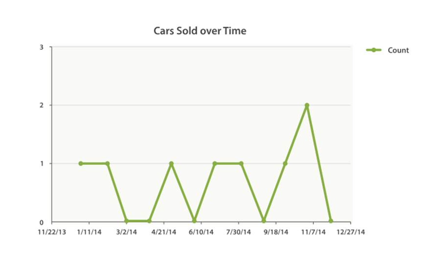
The extended_bounds parameter does just that. Once you add those two settings, you’ll get a response that is easy to plug straight into your graphing libraries and give you a graph like Figure 28-1.

Figure 28-1. Cars sold over time
Extended Example
Just as we’ve seen a dozen times already, buckets can be nested in buckets for more-sophisticated behavior. For illustration, we’ll build an aggregation that shows the total sum of prices for all makes, listed by quarter. Let’s also calculate the sum of prices per individual make per quarter, so we can see which car type is bringing in the most money to our business:
GET /cars/transactions/_search?search_type=count
{
"aggs": {
"sales": {
"date_histogram": {
"field": "sold",
"interval": "quarter", ![]()
"format": "yyyy-MM-dd",
"min_doc_count" : 0,
"extended_bounds" : {
"min" : "2014-01-01",
"max" : "2014-12-31"
}
},
"aggs": {
"per_make_sum": {
"terms": {
"field": "make"
},
"aggs": {
"sum_price": {
"sum": { "field": "price" } ![]()
}
}
},
"total_sum": {
"sum": { "field": "price" } ![]()
}
}
}
}
}
![]()
Note that we changed the interval from month to quarter.
![]()
Calculate the sum per make.
![]()
And the total sum of all makes combined together.
This returns a (heavily truncated) response:
{
....
"aggregations": {
"sales": {
"buckets": [
{
"key_as_string": "2014-01-01",
"key": 1388534400000,
"doc_count": 2,
"total_sum": {
"value": 105000
},
"per_make_sum": {
"buckets": [
{
"key": "bmw",
"doc_count": 1,
"sum_price": {
"value": 80000
}
},
{
"key": "ford",
"doc_count": 1,
"sum_price": {
"value": 25000
}
}
]
}
},
...
}
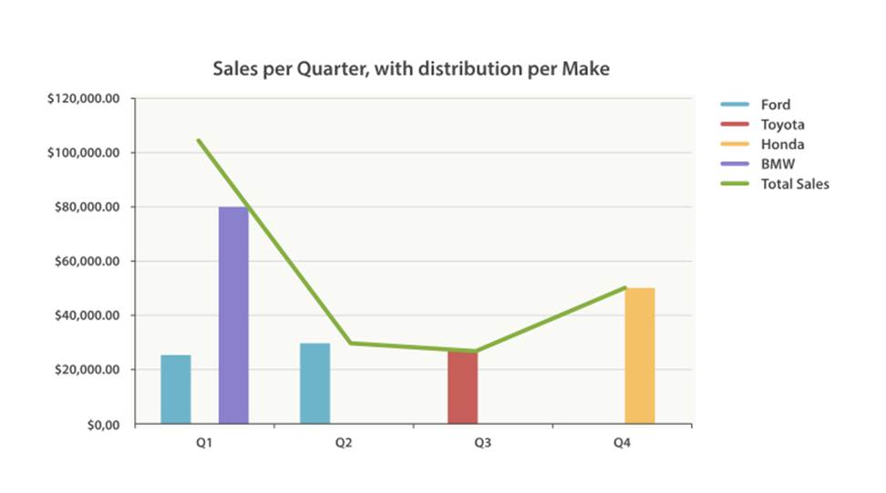
We can take this response and put it into a graph, showing a line chart for total sale price, and a bar chart for each individual make (per quarter), as shown in Figure 28-2.

Figure 28-2. Sales per quarter, with distribution per make
The Sky’s the Limit
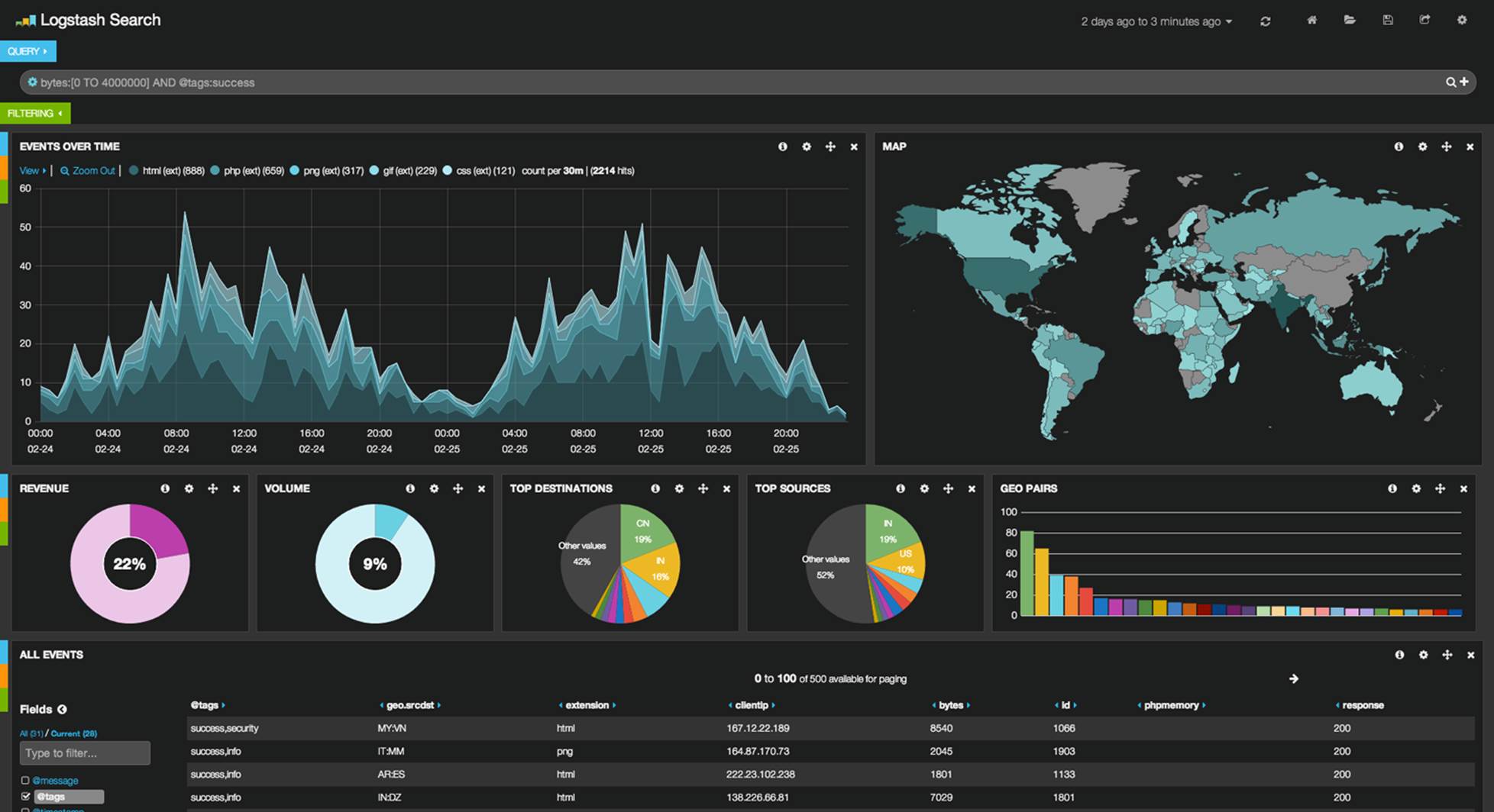
These were obviously simple examples, but the sky really is the limit when it comes to charting aggregations. For example, Figure 28-3 shows a dashboard in Kibana built with a variety of aggregations.

Figure 28-3. Kibana—a real time analytics dashboard built with aggregations
Because of the real-time nature of aggregations, dashboards like this are easy to query, manipulate, and interact with. This makes them ideal for nontechnical employees and analysts who need to analyze the data but cannot build a Hadoop job.
To build powerful dashboards like Kibana, however, you’ll likely need some of the more advanced concepts such as scoping, filtering, and sorting aggregations.
All materials on the site are licensed Creative Commons Attribution-Sharealike 3.0 Unported CC BY-SA 3.0 & GNU Free Documentation License (GFDL)
If you are the copyright holder of any material contained on our site and intend to remove it, please contact our site administrator for approval.
© 2016-2025 All site design rights belong to S.Y.A.