Emerging Trends in Image Processing, Computer Vision, and Pattern Recognition, 1st Edition (2015)

Part I. Image and Signal Processing

Chapter 14. Correction of intensity nonuniformity in breast MR images

S. Yazdani¹; R. Yusof¹; A. Karimian²; M. Pashna¹; A. Hematian^{3 1} Malaysia-Japan International Institute of Technology (MJIIT), Universiti Teknologi Malaysia, Jalan semarak 54100 Kuala Lumpur, Malaysia
² Department of Biomedical Engineering, Faculty of Engineering, University of Isfahan, Isfahan, Iran
³ Department of Computer and Information Sciences, Towson University, Towson, MD, USA

Abstract

Breast cancer is one of the most prevalent cancers among women. Mammography, as one of the primary studies, is used for diagnosis of breast disease. In addition, MR images can depict most of the significant changes of breast during the time. For the first step of breast disease detection, the density measurement of the breast on MR images may provide very useful information. MR images have some instinctive limitations like the strongly dependence of contrast upon the way the image is acquired, noise, partial volumes, intensity inhomogeneities (bias field), etc. For these reasons, an effective normalization on breast MR images is very important issue for detecting breast disease signs. The first important step for quantitative analysis of breast density on MRI is preprocessing step including noise reduction and bias field correction. In this study, N3 algorithm is used for correcting the field inhomogeneity in MR images. We used T1-weighted images, using a 1.5-T MRI scanner. The results demonstrate effectiveness and efficiency of the proposed method.

Keywords

Bias field correction

Breast disease diagnosis

MR images

N3 method

Acknowledgments

The authors would like to thank Ministry of Education of Malaysia (MoE), University Teknologi Malaysia (UTM) and Research Management Centre of UTM for providing financial support under the GUP Research Grant No. 04H40, titled “Dimension reduction and Data Clustering for High Dimensional and Large Datasets.”

1 Introduction

Breast cancer is the second factor for death among women around the world [1]. Mammography is considered as one of the primary studies on tumor diagnosis and breast disease. It is not recommended to have frequent MRIs for high-risk women because of radiation. Scientists are looking for the best way for quantifying breast densities of MR images in healthy women to assessment of healthy breast composition. They are trying to find the link between breast cancer and breast composition. In addition, these assessments can help future researches to estimate potential risk of breast cancer. Our goal is normalizing MR images for quantifying density of the breast accurately, because this factor is an important marker in diagnosis of breast cancer. However, MR images has some limitations, such as, they sometimes are in low contrast, the dependence of MR image quality upon the condition the image is acquired, ideal image situation is never realized practically, bias field, etc.

One of the main problems of MR images is bias field [2]. Bias field has been a challenging problem in MR image segmentation. It is a smooth and low-frequency signal that corrupts MRI images specially those produced via old MRI machines. Bias field is attributed to eddy current, poor radio frequency (RF) coil uniformity, and patient anatomy [3]. Bias field eliminate high-frequency contents of MRI image like contours and edges, blur the images, change the intensity of image pixels, as a result, same tissues have different gray level distribution in the image. In order to decrease the aforementioned restriction, research teams throughout the world have conducted some studies on bias field correction in mammographic images [4,5].

According to their studies there are two main methods for bias field correction: prospective and retrospective methods. The prospective methods try to solve this problem in the process of acquisition by using special hardware. These approaches can only delete inhomogeneities due to hardware imperfections.

Retrospective approaches have been more developed; they are classified into two groups: first group uses the segmentation-based methods for computing the bias field and the second one works directly on data.

Although the segmentation-based approaches, such as expectation maximization (EM) algorithm [6], FCM-based methods [7,8], maximum likelihood [9,10], and MAP-based approaches [11,12], have obtained suitable result, they have some disadvantages such as: they work solely on intensity of image and they are able only to estimate and correct low amplitude intensity inhomogeneities [13].

These methods work directly on MRI image data such as SPM99 [14]. These methods has a problem of entropy minimization. Another method in this category is N3 (nonparametric intensity nonuniformity normalization) [3], which we used it in this chapter for bias field correction. N3 method was determined to be the best method on the recent studies [3].

After digitalizing the images, N3 method was used for bias field estimation and correction. The input of proposed method includes different percentages of intensity inhomogeneities, while the output consists of bias field corrected images with very high quality, which indicate breast regions more precisely.

2 Preprocessing steps

The main purpose of the preprocessing stage is to enhance the image quality for further processing steps by reducing or correcting the unrelated artifacts in the mammogram images. Mammograms image analysis is problematic due to existence of different artifacts that make the processing step complicated. Therefore, preprocessing stage is essential to improve the image quality. It will prepare the mammogram image for the next processing stages.

2.1 Noise Reduction

Magnetic resonance images are corrupted by Rician distribution that arises from complex Gaussian noise in the original frequency domain measurements.

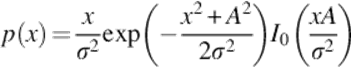
The Rician probability density function for the corrupted MR image intensity x is demonstrated as follows:

(1)

where σ is the standard deviation of the noise, A is the underlying true intensity, and I₀ is the modified Bessel function of the first kind with order zero [15]. Median filter is one of the most popular nonlinear spatial filters for noise reduction that is more efficient than convolution when the purpose is to preserve borders and decrease noise simultaneously. This method is simple, computationally efficient, and also has a well denoizing power.

The median filter replaces the value of a given pixel with the median pixel value within a region of interest. A median filter with properly selected window size can smooth the noise in the original image. It may also virtually eliminate the main tissues information from the MR image. Therefore, there will be a trade-off between noise reduction and the preservation of information from image. Clearly, by increasing the size of the median window, both noise signals and signals from main tissues are being suppressed. For the 7 × 7 case, it removed more of the useful information than the 5 × 5 case. Therefore, the 5 × 5 median is the best for noise removal and preservation of brain tissue information [16].

The operation of median filtering technique is presented as:

(2)

Let Sxy and median be the set of coordinates in a subimage window which is centered at (x,y) and the median value of the window, respectively.

2.2 Bias Field Reduction

It is also called intensity inhomogeneity or intensity nonuniformity, which is one of the main problematic and challenging issues in MRI. It is a low-frequency undesirable signal that blurs MR images and thus decreases the high-frequency contents of MRI such as contours and edges.

Bias field is not always visible to the human eye and has a negative effect on segmentation results. For analysis techniques such as image segmentation, the presence of intensity nonuniformity may reduce its reliability and accuracy dramatically, as per the hypothesis that intensity is uniform in each tissue class being no longer verified.

Thus, the correction of intensity nonuniformity can improve the application of many quantitative analyses.

Bias field is the smooth intensity variation in MR images caused by different factors such as:

• Nonuniform reception sensitivity

• Inhomogeneous RF

• Nonuniform reception sensitivity

Other less important parameters causing the bias field include:

• Eddy currents

• Mistuning of the RF coil

• Geometric distortion

• Patient movement

These parameters cause intensity variation over the image and the totality of the imaged object [17]. Different methods exist to compensate for the inhomogeneity problem [18–22]. The aim of this study is to show how to restore the corrupted image for MR images that corrupted by bias field. We used two-step normalization method.

2.3 Locally Normalization Step

One of the problems, which happen in quantitative analysis of MRI, is that the results are not comparable between consecutive scans, different anatomical regions and within the same scan.

In order to segment MRI images in an effective approach, undesirable signals must be suppressed before segmentation process. Thus, one of the major challenges is eliminating the bias field. A normalization filter is required to remove low-frequency magnetic field variations within the MR images in order to regulate image brightness and contrast while preserving details.

In our normalization method, a sliding window is applied to slide vertically on each MRI image to compensate the current image bias field effects through histogram analysis.

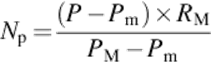
In order to calculate the normalization factor, all the pixels within the region of the sliding window are gathered as the input data. Then the standard deviation of all gathered pixel values is calculated (SD1) beside the standard deviation of the mid-line of the sliding window (SD2). All the pixel data in the mid-line need to be shifted to the desired offset where the SD2 meets the SD1 value. At this point, the difference in the SD1 and SD2 is added to the pixel values of the mid-line to compensate the bias field effect. When the minimum and maximum pixel values of the mid-line are obtained, the mid-line pixel data are then stretched to its maximum data resolution (8-bit, 0–255) where the minimum value is zero and the maximum value is 255 (see Equation 3):

(3)

where N_p is the normalized pixel value, p is the pixel value, P_m is the minimum pixel value in the image, P_M is the maximum pixel value in the image, and R_M is the maximum value of pixel bit depth.

In this step, a locally normalization via a resizable sliding window is performed to compensate intensity nonuniformity in MR images.

2.4 Hybrid Method for Bias Field Correction

Nonparametric intensity nonuniformity normalization (N3) was proposed by Sled et al. [3] for solving the problem of artifacts in MRI images. It is an iterative method, which estimates multiplicative bias field and true tissue intensity distribution. This method is an intensity model-based or histogram-based approach. Unlike some other methods such as EM, N3 does not rely on tissue classification.

One of the main advantages of nonparametric methods is that they do not make any assumptions about the patient anatomy. In addition, it is fully automatic, accurate, and robust method. In this step, a combination of N3 algorithm and singularity function analysis (SFA) model is used in breast MR images.

2.4.1 Bias field model

The following equation is the basis of the N3 method [23]. Bias field is often modeled as a multiplicative field:

(4)

In which, f is an unknown bias field or intensity inhomogeneity, v is the observed image, x designates the spatial position or voxel, u is the true image, and n is the noise which assumed to be independent of u.

The main stage for correcting bias field is estimating its distribution (f). The mixture of multiplicative and additive model makes this stage difficult.

The challenging problem of bias field correction consists of recovering u(x) from information about the multiplicative factor f(x) and the additive term n(x). Due to the simultaneous presence of n(x) and f(x), it is difficult to solve the problem. Thus, a common solution is to neglect the n(x) that is an additive noise. For the two-dimensional discrete image case and using a log transform, the bias field is made additive.

Consider a case without noise in which u and f are independently distributed random variables. Instead of v, u, f, we deal with log v, log u, log f, then the formation model becomes additive:

(5)

Let V(u,v), U(u,v), and F(u,v) present the probability densities of v(i,j), u(i,j), and f(i,j), respectively. Equation (5) can be expressed as

(6)

Making the approximation that ln u and ln f are uncorrelated random variables, Equation (6) is found by convolution as follows:

(7)

The multiplication corrupts the field and a division can undo the corruption. In the frequency domain, multiplications and divisions convert to convolutions and deconvolutions as follows:

(8)

In which V, U, and F are probability densities. After this stage, the uniformity distribution (F) is modeled and viewed as blurring intensity distribution U that is the main stage for correcting bias field.

2.4.2 Correction step

An straightforward technique for image bias field correction would be that if the spatial frequencies of u(i,j) (the true image) and f(i,j) bias field are disjointed, the bias field can be removed by filtering out the spatial frequencies illustrating the bias field. In some cases, useful knowledge in MRI related to higher spatial frequencies than the intensity nonuniformity. Thus, by removing low spatial frequencies, intensity nonuniformity can be suppressed. The problem is that in most cases, spatial frequency information of the bias field and true image are not perfectly separated, and they have some overlapped components. For example, in MRI scans, when low spatial frequencies are removed, the spatial image will be considerably changed, implying the existence of useful knowledge at low spatial frequency bands. In such situations, using low pass filtering eliminates not only bias field but also useful knowledge in the true image, therefore decreasing the quality of the bias field corrected breast image. Another group of bias field correction methods relies on the assumption that anatomical knowledge in MRI occurs in the higher spatial frequency bands than intensity nonuniformity. These methods remove the bias field by filtering out highest spatial frequency bands demonstrating anatomical knowledge. One of the disadvantages of these methods is that the results depend on anatomy.

In this chapter, we used SFA idea [17], which assumes that anatomical information of MRI occurs in the high spatial frequencies in the image. In this method, after low pass filtering, since useful low spatial frequencies are removed during the filtering process, the filtered version of the ideal signal does not look like the original unbiased signal. SFA models recover the removed low-frequency information via reconstructing spatial information from the rest of high spatial frequencies.

In general, we applied a model that uses the assumption that bias field does not corrupt high spatial frequency bands in the image. Consequently, we first removed all low spatial frequencies without recognizing important information. Second, we recreated the spatial image from the remained higher spatial frequencies. The low spatial frequencies, which are related to intensity nonuniformity, are thus removed in the recreated image, leading to an intensity nonuniformity corrected breast image.

2.4.3 Field estimation

Using the distribution of U, we can estimate bias field estimation as follows. For a measurement at some location x, can be estimated using the distributions F and U ( = [log(u)]).

The estimated value of given a measurement v_j is defined as follows:

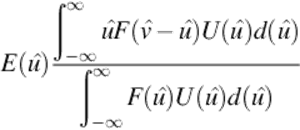(9)

By using the estimation of , the estimation of f can be found as follows:

(10)

where is the estimation of f_e, based on the single measurement of at location x.

The difference between v and computed expectation of real signal, given the measured signal. Finally, the distribution U is estimated applying a deconvolution filter as follows:

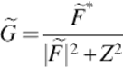(11)

In which * defines complex conjugate, is the Fourier transform of F, Z is a constant term for limiting the magnitude of G.

This estimation is then used to estimate a corresponding field.

In addition to processing stages were described above, there are some steps for practical impletion of applied algorithm.

• Estimating V distribution by using an equal-size bins histogram and Parzen window [24].

(12)

(13)

In which h is the distance between , x_i is the location, N is the set of measurements v(x_i), is the centers of the bins

• Smoothing the bias field by using the B-spline technique [25]. For doing this stage, the MRI data should resample into subsamples (coarser resolution). This step is carried out because smoothing the bias field at full resolution is computationally difficult.
The smoothing stage is a challenging stage and the manner of smoothing, effects on bias field correction performance. The proposed approach for smoothing is approximating data by using linear combination of smooth basis functions. B-spline is a suitable basis, which is compactly supported spline. In comparison with conventional filtering approaches the proposed technique is superior regarding to missing data. Filtering methods are not suitable for this step because of boundary effects, which degraded overall performance substantially. The boundary of the chest wall of fatty tissues may be smoothed out to be close to outside background [13].

• Resampling to original resolution and using it for correcting original volume.

• Terminating the iterations using the variation coefficient, as follows:

(14)

where rn is the ratio between subsequent field estimates at the location, б is the standard deviation, and μ is the mean.

When e falls below determined threshold, the iteration is stopped. In this chapter, breast MR images including variety percentages of bias field were used.

By using mentioned method, the bias field is removed and the specialist can assess and quantify the density of the breast accurately, and also the bias field corrected images are ready for another processing such as segmentation.

More importantly, segmentation and bias field estimation are mutually influenced by each other and the performance of MRI segmentation can be degraded significantly by the presence of bias field. If the bias field is corrected, the segmentation would be more powerful and it helps to specialist to have an accurate assessment.

3 Experimental Results

This chapter demonstrated recent progress on MR image bias field correction. As mentioned above there are different methods, which are popular to bias field correction such as low pass filtering and statistical methods. Low pass filtering techniques are fast, easy to code, in addition, they can also be adaptive to image data. One of the main disadvantages of low pass filtering method is assuming the bias field as low-frequency signal. This methods also assume that the other image component have higher frequency, which is usually wrong for some cases. In addition, they tend to corrupt low-frequency components in tissue.

Statistical techniques are easy to integrate with other knowledge such as registration, segmentation, or some image feature but one of the disadvantages of these methods is that they often have relied on Gaussian distribution for modeling the intensity distribution of tissues, but experimental results show that intensity distribution of tissue do not indicate a Gaussian mixture exactly. This method fails to present some tissues [26].

Overall, the N3 method is superior to the other methods in robustness and high performance point of view [27].

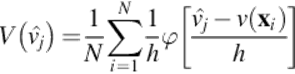
In this part, we show the efficacy of proposed algorithm for clinical breast MRIs. All of the images were acquired by 1.5 T clinical MR scanner in “Isfahan radiology Medical Center.” Figure 1(a) demonstrates a breast MR image corrupted by bias field and bias field corrected image using mentioned algorithm.

FIGURE 1 From left to right: (a) Original MR image with severe bias field, (b) Estimated bias field and (c) Corrected image.

Mentioned algorithm estimated bias field, corrected it, and improved the image contrast and quality dramatically. Figure 2 indicates other examples of breast MRI.

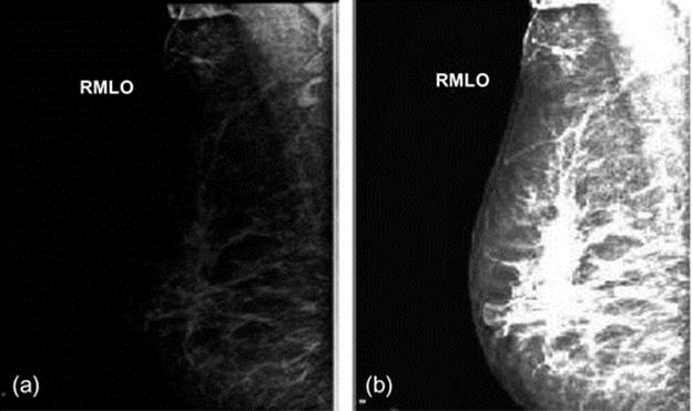
FIGURE 2 From left to right: (a) Original MR image, (b) corrected image.

We can see that the bias field in our clinical database is 30–40% and the algorithm has removed the bias field successfully.

In Figures 1 and 2, MRI digitalized images have different percentages of bias field. These images are blurred because of bias field existence and breast compositions are not clearly shown. In the images, which are normalized through mentioned algorithm, these regions are presented clearly in Figures 1(c) and 2(b). In these images, the dynamic range is increased and the fatty tissues became brighter than before and they can be separated from fibroglandular tissues.

4 Conclusion

The bias field is the challenging problem of MR images. It changes the intensity values of pixels in MRI image and corrupts these images. The correction of this problem is necessary for subsequent computerized quantitative analysis. The high importance of bias field correction, motivated us to use a fast, reliable, and robust algorithm to solve this problem. It is expected that a fully automated algorithm for bias field correction in breast MRI may have great potential in clinical MRI applications.

In this chapter, an effective, robust, and accurate method is used for bias field correction in breast MR images. We proposed a new combination of locally normalization, N3, and SFA methods. The proposed technique takes advantage of N3 and SFA methods and not only preserves simplicity, but also has the potential to be generalized to multivariate versions adapted for segmentation applying multimodality images (e.g., T1, T2, and PD images). N3 method is an iterative algorithm and does not need any model assumption. This method does not rely on any prior knowledge of pathological data as a result can be applied at early stage and it is a substantial advantage in automated data analysis. Breast MRI image as an input enters into the proposed package and after different processing steps, the output is an image which indicates breast compositions and density measurement of the breast. The efficacy of the algorithm is presented on clinical breast MRIs and the results show the potential of method to extract useful information for breast disease detection. Extension of this method for tumor and disease detection is the next challenging task for the future.

References

[1] Avril N, Schelling M, Dose J, Weber WA, Schwaiger M. Utility of PET in breast cancer. Clin Positron Imaging. 1999;2:261–271.

[2] Roy S, Carass A, Bazin PL, Prince JL. Intensity inhomogeneity correction of magnetic resonance images using patches. In: SPIE 7962, Medical imaging. 2011:9621F.

[3] Sled JG, Zijdenbos AP, Evans AC. A nonparametric method for automatic correction of intensity nonuniformity in MRI data. IEEE Trans Med Imaging. 1998;17:87–97.

[4] Kim K, Habas P, Rajagopalan V, Scott J, Rousseau F, Glenn O, et al. Bias field inconsistency correction of motion-scattered multislice MRI for improved 3D image reconstruction. IEEE Trans Med Imaging. 2011;30.

[5] Wels M, Zheng Y, Huber M, Hornegger J, Comaniciu D. A discriminative model-constrained EM approach to 3D MRI brain tissue classification and intensity non-uniformity correction. Phys Med Biol. 2011;56:3269.

[6] Dempster AP, Laird NM, Rubin DB. Maximum likelihood from incomplete data via the EM algorithm. J R Stat Soc Series B Stat Methodol. 1977;1–38.

[7] Pham DL, Prince JL. An adaptive fuzzy C-means algorithm for image segmentation in the presence of intensity inhomogeneities. Pattern Recognit Lett. 1999;20:57–68.

[8] Clarke L, Velthuizen R, Camacho M, Heine J, Vaidyanathan M, Hall L, et al. MRI segmentation: methods and applications. Magn Reson Imaging. 1995;13:343–368.

[9] Van Leemput K, Maes F, Vandermeulen D, Suetens P. Automated model-based bias field correction of MR images of the brain. IEEE Trans Med Imaging. 1999;18:885–896.

[10] Gispert JD, Reig S, Pascau J, Vaquero JJ, García-Barreno P, Desco M. Method for bias field correction of brain T1-weighted magnetic resonance images minimizing segmentation error. Hum Brain Mapp. 2004;22:133–144.

[11] Wells III W, Grimson W, Kikinis R, Jolesz F. Adaptive segmentation of MRI data. IEEE Trans Med Imaging. 1996;15:429–442.

[12] Guillemaud R, Brady M. Estimating the bias field of MR images. IEEE Trans Med Imaging. 1997;16:238–251.

[13] Manjón JV, Lull JJ, Carbonell-Caballero J, García-Martí G, Martí-Bonmatí L, Robles M. A nonparametric MRI inhomogeneity correction method. Med Image Anal. 2007;11:336–345.

[14] Ashburner J, Friston KJ. Voxel-based morphometry—the methods. Neuroimage. 2000;11:805–821.

[15] Nobi M, Yousuf M. A new method to remove noise in magnetic resonance and ultrasound images. J Sci Res. 2011;3.

[16] Singh WJ, Nagarajan B. Automatic diagnosis of mammographic abnormalities based on hybrid features with learning classifier. Comput Methods Biomech Biomed Eng. 2013;16:758–767.

[17] Luo J, Zhu Y, Clarysse P, Magnin I. Correction of bias field in MR images using singularity function analysis. IEEE Trans Med Imaging. 2005;24:1067–1085.

[18] Ivanovska T, Laqua R, Wang L, Völzke H, Hegenscheid K. Fast implementations of the levelset segmentation method with bias field correction in MR images: full domain and mask-based versions. In: Berlin, Heidelberg: Springer; 674–681. Pattern recognition and image analysis. 2013;vol. 7887.

[19] Adhikari SK, Sing J, Basu D, Nasipuri M, Saha P. Segmentation of MRI brain images by incorporating intensity inhomogeneity and spatial information using probabilistic fuzzy c-means clustering algorithm. In: International Conference on Communications, Devices and Intelligent Systems (CODIS); 2012:129–132 2012.

[20] Fletcher E, Carmichael O, DeCarli C. MRI non-uniformity correction through interleaved bias estimation and B-spline deformation with a template. In: 2012 Annual International Conference of the IEEE Engineering in Medicine and Biology Society (EMBC); 2012:106–109.

[21] Verma N, Cowperthwaite MC, Markey MK. Variational level set approach for automatic correction of multiplicative and additive intensity inhomogeneities in brain MR Images. In: 2012 Annual International Conference of the IEEE Engineering in Medicine and Biology Society (EMBC); 2012:98–101.

[22] Uwano I, Kudo K, Yamashita F, Goodwin J, Higuchi S, Ito K, et al. Intensity inhomogeneity correction for magnetic resonance imaging of human brain at 7T. Med Phys. 2014;41:022302.

[23] Lin M, Chan S, Chen JH, Chang D, Nie K, Chen ST, et al. A new bias field correction method combining N3 and FCM for improved segmentation of breast density on MRI. Med Phys. 2011;38:5.

[24] Gao G. A parzen-window-kernel-based CFAR algorithm for ship detection in SAR images. IEEE Geosci Remote Sens Lett. 2011;8:556–560.

[25] Csébfalvi B. An evaluation of prefiltered B-spline reconstruction for quasi-interpolation on the body-centered cubic lattice. IEEE Trans Vis Comput Graph. 2010;16:499–512.

[26] Lee JD, Su HR, Cheng PE, Liou M, Aston J, Tsai AC, et al. MR image segmentation using a power transformation approach. IEEE Trans Med Imaging. 2009;28:894–905.

[27] Hou Z. A review on MR image intensity inhomogeneity correction. Int J Biomed Imaging. 2006;2006:1–11.