Emerging Trends in Image Processing, Computer Vision, and Pattern Recognition, 1st Edition (2015)
Part II. Computer Vision and Recognition Systems
Chapter 30. Detecting distorted and benign blood cells using the Hough transform based on neural networks and decision trees
Hany A. Elsalamony Mathematics Department, Faculty of Science, Helwan University, Cairo, Egypt
Abstract
Sickle-cell anemia is one of the most important types of anemia. This paper presents an algorithm for detecting blood cells characteristic of sickle-cell anemia. First, I discuss the construction of an algorithm that can be used to detect and count benign or distorted red blood cells (RBCs) in a microscopic colored image, even if those cells are hidden or overlapped. Second, I explain the process for checking and analyzing the constructed RBC data by applying two important techniques in data mining: the neural network (NN) and the decision tree. I then review experiments demonstrating that these models show high accuracy when predicting the counts of benign or distorted cells. In these experiments, the algorithm has segmented around 99.98% of all input cells, helping to improve the diagnosis of sickle-cell anemia. The NN has shown a 96.9% agreement with the algorithm’s prediction outcomes, and the classification and regression tree has achieved 92.9%.
Keywords
Sickle-cell anemia
Image watershed segmentation
Red blood cell detection and counting
C&R tree
Neural network
1 Introduction
Naturally, the human blood consists of a complex combination of plasma, red blood cells (RBCs), white blood cells (WBCs), and platelets. Plasma is the fluid component, which contains melted salts and proteins. RBCs make up about 40% of blood volume. WBCs are less, but greater in size than RBCs. The platelet cells are similar particles, which are smaller than WBCs and RBCs [1].
Anemia occurs when the blood has lower than the normal number of RBCs or insufficient hemoglobin. RBCs are made inside the spongy marrow of the body’s larger bones. Bone marrow is always making new RBCs to replace old ones. Normal RBCs die after 120 days in the bloodstream. Their job is carrying oxygen and removing carbon dioxide (a waste product) from the body. In addition, RBCs are disk-shaped and move easily through blood vessels, and they contain an iron-rich protein called hemoglobin. This protein transmits oxygen from the lungs to the rest of the body [1]. In sickle-cell anemia, the body makes sickle-shaped RBCs. Sickle cells contain abnormal hemoglobin called sickle hemoglobin or hemoglobin S, which contributes to the cells developing a sickle, or crescent, shape. Sickle cells are very dangerous because of their rigidity and stickiness, which cause the cells to clump, blocking blood flow in the blood vessels of the limbs and organs. The blocked blood flow can cause pain, organ damage, and increased probability of infection. Moreover, the abnormal sickle cells usually die after only about 10-20 days, and the bone marrow cannot make new RBCs fast enough to replace the dying ones [1]. Figure 1 illustrates the danger of sickle-cell anemia and its various types.
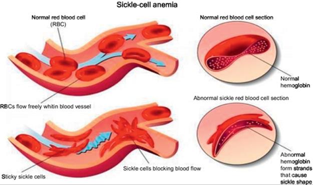
FIGURE 1 Kinds of RBCs and sickle-cell anemia.
Sickle-cell anemia is most common in people whose families originate from Mediterranean countries, Africa, South or Central America (especially Panama and the Caribbean islands), Saudi Arabia, and India. In the United States of America, approximately 70,000 to 100,000 people suffer from the condition, and they are mainly African Americans. The discovery of this disease depends on blood test analysis that can specifically detect sickle cells [1].
Recently, microscopic-image analysis has been used as an impressive diagnostic tool for detecting irregular blood cells [1]. The Hough transforms is the most important technique applied to image analysis and segmentation for the detection of blood cells. The transform depends on extracting features related through the segmentation of the microscopic image. Generally, the Hough transforms used today were invented by Richard Duda and Peter Hart in 1972, who called it a “generalized Hough transforms” after the related 1962 patent of Paul Hough [2,3]. Figure 2 shows a simple example of a pixel lying on a definite circle (solid circle), and the classical circular Hough transform (CHT) voting pattern (dashed circles) for the applicant pixel.
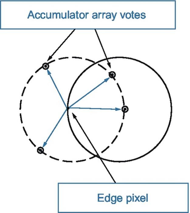
FIGURE 2 Voting in classic circular Hough transforms.
On the other hand, data mining techniques have gained popularity as illustrative and predictive applications of image analysis, and researchers have used the two techniques on blood cell detection data. The neural network (NN) is one of these techniques, and it has been successfully applied in the identification and control of dynamic systems. In 1986, David Rumelhart introduced concepts related to the NN when he presented a back-propagation process, which used many layers throughout the network.
Another technique of data mining is the classification and regression tree (C&R), which is the most common and powerful technique for classifying data and predicting outcomes in the decision tree (DT). It can generate understandable rules and handle both continuous and categorical variables [4]. The C&R tree algorithm had been popularized by Breiman, Friedman, Olshen, and Stone in 1984, before Ripley in 1996 [5]. The popularity of DT techniques is due to two features: (1) the procedures are relatively straightforward to understand and explain, and (2) the procedures address a number of data complexities, such as nonlinearly and interactions, that commonly occur in real data [4].
This chapter is divided into two parts. In the first part, I apply a proposed algorithm to detect benign and distorted blood cells (sickle-cell anemia) and to count them depending on the segmentation of their shapes using CHT, watershed, and morphological tools. In the second part, I introduce an algorithm for checking and analyzing the resulting cell data variables (e.g., area, convex area, perimeter, and eccentricity) by applying the most important techniques in data mining, NN and DT (C&R tree), to get the right decision for diagnosis [6].
To this end, the chapter is organized as follows: Section 2 focuses on the related work which is presenting a literature review on the work in this chapter, and Section 3 presents the definition and features of the Hough transform. Section 4 provides an overview of the NN. Section 5 discusses the C&R of DTs, and the proposed algorithm is presented in Section 6. In Section 7, the experimental results show the effectiveness of each model, and I offer a conclusion in Section 8.
2 Related work
In recent years, research on the blood cells' detection and diagnosis of diseases using image processing has grown rapidly. In 2010, Y M Hirimutugoda and Gamini Wijayarathna presented a method to detect thalassaemia and malarial parasites in blood sample images acquired from light microscopes and investigated the possibility of rapid and accurate automated diagnosis of red blood cell disorders. To evaluate the accuracy of the classification in the recognition of medical image patterns, they trained two back propagation Artificial Neural Network models (3 layers and 4 layers) together with image analysis techniques on morphological features of RBCs. The three layers had the best performance with an error of 2.74545e-005 and 86.54% correct recognition rate. The trained three layer ANN acts as a final detection classifier to determine diseases [7].
In December 2012, D.K. DAS, C. CHAKRABORTY, B. MITRA, A.K. MAITI, and A.K. RAY introduced a methodology using some techniques of machine learning for characterizing RBCs in anemia based on microscopic images of peripheral blood smears. In the first, for reducing unevenness of background illumination and noise they preprocessed peripheral blood smear images based on geometric mean filter and the technique of gray world assumption. Then watershed segmentation technique applied to erythrocyte cells. The distorted RBCs, such as, sickle cells, echinocyte, tear drop, acanthocyte, elliptocyte, and benign cells have been classified as dependent on their morphological shape changes. They observed that when a small subset of features used by using information gain measures, the logistic regression classifier presented better in performance. They achieved highest prediction in terms of overall accuracy by 86.87%, sensitivity to 95.3%, and specificity was 94.13% [8].
In May 2013, Thirusittampalam, Hossain, Ghita, and Whelan developed a novel tracking algorithm that extracted cell motility indicators and determined cellular division (mitosis) events in large time-lapse phase-contrast image sequences. Their process of automatic, unsupervised cell tracking was carried out in a sequential manner, with the interframe cell's association achieved by assessing the variation in the local cellular structures in consecutive frames from the image sequence. The experimental results indicated that their algorithm achieved 86.10% overall tracking accuracy and 90.12% mitosis detection accuracy [9].
Also in May 2013, Khan and Maruf presented an algorithm for cell segmentation and counting via the detection of cell centroids in microscopic images. Their method was specifically designed for counting circular cells with a high probability of occlusion. The experimental results showed an accuracy of 92% of cell counting, even at around 60% overlap probability [10].
An algorithm presented by Mushabe, Dendere, and Douglas in July 2013 identified and counted RBCs as well as parasites in order to perform a parasitemia calculation. The authors employed morphological operations and histogram-based thresholds to detect the RBCs, and they used boundary curvature calculations and Delaunay triangulation to split overlapped cells. A Bayesian classifier with their RGB pixel values as features classified the parasites, and the results showed 98.5% sensitivity and 97.2% specificity for detecting infected RBCs [11]. In 2014, Rashmi Mukherjee presented an evaluation the morphometric features of placental villi and capillaries in preeclamptic and normal placentae. The study included light microscopic images of placental tissue sections of 40 preeclamptic and 35 normotensive pregnant women. The villi and capillaries characterized based on preprocessing and segmentation of these images. He applied principal component analysis (PCA), Fisher’s linear discriminant analysis (FLDA), and hierarchical cluster analysis (HCA) to identify placental (morphometric) features, which are the most significant from microscopic images. He achieved 5 significant morphometric features (>90% overall discrimination accuracy) identified by FLDA, and PCA returned three most significant principal components cumulatively explained 98.4% of the total variance [12]. From this literature survey, it was noticed that research work has been done towards anemia-affected RBCs’ characterization using computer vision approach. The proposed work methodology has described in Section 6.
3 Hough transforms
The Hough transform is a popular feature extraction technique that converts an image from Cartesian to polar coordinates. Any point within the image space is represented by a sinusoidal curve in the Hough space. In addition, two points in a line segment generate two curves, which are overlaid at a location that corresponds with a line through the image space. Even though this model form is very easy, it is deeply complicated for the case of complex shapes due to noise and shape imperfection, as well as the problem of finding slopes of vertical lines. The CHT solved this problem by putting a transformation of the centroid of the shape in the x-y plane to the parameter space [13].
There are three essential steps common to all CHTs. First, a CHT contains an accumulator array computation of high gradient foreground pixels, which chosen as candidate pixels. Then they are collected “votes” in the accumulator array. Center estimation is the second step. It predicts the circles centers by detecting the peaks in the accumulator array that produced through voting on candidate pixels. The votes are accumulated in the accumulator array box according to a circle’s center. Figure 3 shows an example of the candidate pixels (solid dots) falling on an actual circle (solid circle), as well as their voting patterns (dashed circles), which coincide with the center of the substantial circle. The third step in a CHT is radius estimation; if the same accumulator array has been used for more than one radius value, as is commonly done in CHT algorithms, the radii of detected circles must be estimated as a separate step [2]. The radius can be clearly estimated by using radial histograms; however, in phase-coding, the radius can be estimated by simply decoding phase information from the estimated center located within an accumulator array [2]. For this chapter, I have used a CHT to detect and count RBCs, even if they are hidden or overlapped. Watershed and morphological functions are used to enhance and separate overlapped cells during the segmentation process.
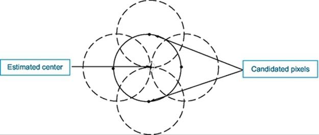
FIGURE 3 Circle center estimated.
4 Overview of NN
Now, NN with back propagation is the most popular artificial NN construction, and it is known as a powerful function approximation for prediction and classification problems. Historically, the NN has been viewed as a mutually dependent group of artificial neurons that uses a mathematical model for information processing, with a connected approach to computation introduced by Freeman in 1991 [4,14]. The NN structure is organized into layers of input, output neurons, and hidden layers, as in Figure 4.
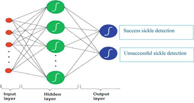
FIGURE 4 The structure of a neural network.
The activation function may be a simple threshold function, a sigmoid hyperbolic tangent, or a radial basis function [15].
![]() (1)
(1)
Back propagation is a common training technique for an NN. This training process requires the NN to perform a particular function by adjusting the values of the connections (weights) between elements [6,16]. Actually, three important issues related to the NN need to be addressed: selection of data samples for network training, selection of an appropriate and efficient training algorithm, and determination of network size [17,18].
Moreover, an NN has many advantages, such as the good learning ability, less memory demand, suitable generalization, fast real-time operating, simple and convenient utilization, adeptness at analyzing complex patterns, and so on. On the other hand, an NN has some disadvantages, including its requirement for high-quality data, the need for careful a priori selection of variables, the risk of over-fitting, and the required definition of architecture [14].
5 Overview of the classification and regression tree
C&R trees are the most common and popular nonparametric DT learning technique. In this chapter, I only use a regression tree for numeric data values. C&R builds a binary tree by splitting the records at each node according to a function of a single input variable. The measure used to evaluate a potential splitter is diversity. This method uses recursive partitioning to split the training records into segments with similar output variable values [4]. Moreover, the impurity used at each node can be defined in the tree by two measures: entropy, as in Equation (2), and Gini, which has been chosen for this chapter. The equation for entropy follows.
![]() (2)
(2)
The Gini index, on the other hand, generalizes the variance impurity, which is the variance of distribution related to the two classes. As in Equation (3), the Gini index can also be useful as the expected error rate if the class label is randomly chosen from the class distribution at the node. In such a case, this impurity measure would have been slightly stronger at equal probabilities (for two classes) than the entropy measure. The Gini index, which is defined by the following equation, holds some advantages for an optimization of the impurity metric at the nodes [19].
![]() (3)
(3)
When the cases in a node are evenly distributed across the categories, the Gini index takes its maximum value of 1−(1/k), where k is the number of categories for the target attribute. Furthermore, for all cases in the node that belong to the same category, the Gini index equals zero.
6 The proposed algorithm
The goal of this chapter is to describe a process for detecting and distinguishing between benign and distorted blood cells in a colored microscopic image. This work can help doctors, physicians, chemists, and anyone else who cares about blood cell detection and analysis, and determination of diseases. The proposed algorithm is divided into two steps, as shown in Figure 5.
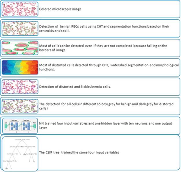
FIGURE 5 The main points of the proposed algorithm.
In the first step, I apply a CHT with morphological functions to the bright and dark intensity of cells to detect and count benign and distorted blood cells. In the second step, I use NN and a C&R tree to test and check the performance of the proposed algorithm for diagnosing a patient with sickle-cell anemia, evaluating which process is more effective than the other. Classification and prediction depend on the detected cells' data variables (e.g., area, convex area, perimeter, and eccentricity) to reduce the errors in detection operation and ensure final diagnosis of sickle-cell anemia. The first part of the CHT includes many operations:
• Cell polarity indicates whether the circulating blood cells are brighter or darker than the background.
• Computation (two-stage) calculates the accumulator array of the CHT. It is based on computing radial histograms; radii are clearly applying the estimated cell centers along with the image information [20].
• The sensitivity factor is the sensor of the accumulator array in the CHT. Detection includes weak and partially hidden or overlapped cells; however, higher sensitivity values increase the risk of false detection.
This stage also determines the edge gradient threshold, given that cells generally have a darker interior (nuclei) surrounded by a bright halo. The edge gradient threshold is very useful for determining edge pixels, and both unhealthy and strong blood cells can be detected based on their contrast by setting a lower value in the threshold. The system detects fewer cells with weak edges when the value of the threshold is increased [15].
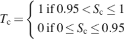
The final stage is the segmentation process, which displays the input image with all the contoured benign (gray) and distorted (dark gray) RBCs. Through this operation, the area, convex area, perimeter, and eccentricities for each cell are measured. In addition, the good and distorted cells can be counted, and the patient can be diagnosed with sickle-cell anemia. These measures are used as input variables to train the NN and C&R tree; but the output (target) measured based on the solidity (S), which it is the area of cell divided by its convex area, as in Equation (4):
![]() (4)
(4)
 (5)
(5)
where areac is the area in each cell, and convex areac represents its convex area for all detected cells (benign and distorted). The target Tc can have two values, 1 and 0, based on the solution of Equation (4). As a result, if any solidity value Sc is > 0.95 up to 1 (perfect cell), Tc takes the value 1 with the decision benign. On the other hand, if Tc takes the value 0, then the Sc value is ≤ 0.95 according to Equation (4), with the decision that the cell is distorted and may be sickled.
The back-propagation NN has been trained and tested using 4 variables as an input layer, 10 neurons in the hidden layer, and 1 neuron in the output layer. Moreover, three kinds of samples are applied: training, validation, and testing samples. The samples are presented in the network during the training process by 80% and 20% for testing process, and the network is modified according to the error. Accordingly, only 10% are used for the validation samples to measure network generalization and to pause training when generalization stops improving. The remaining 10% of all cell samples are introduced as a testing sample that has no effect on training and thus provides an independent measure of network performance during and after training. In addition, the mean square error (MSE) is applied, with the MSE defined as the average squared difference between outputs and targets. For the MSE, lower values are better, and zero means no error. Table 1 illustrates the description of the formed cells' data, which is automatically computed for all cells (benign and distorted).
Table 1
Blood cell variables
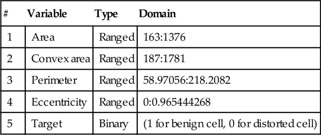
Apart from the NN, the recursive binary C&R tree has been applied to the term of regression because all variables contain numeric values, as shown in Table 1. In this table, all variables range in type, and only the output (target) variable has binary values (e.g., 1 for benign cells and 0 for distorted cells). The binary tree is divided into two branches based on the Gini index and recursively trained with a maximum tree depth of five levels, and it stops when it achieves a parent branch minimum of 2% and a child branch minimum of 1%.
Finally, the performance of each classification model is evaluated using three statistical measures: classification accuracy, sensitivity, and specificity. These measures are defined as true positive (TP), true negative (TN), false positive (FP), and false negative (FN). A TP decision occurs when the positive prediction of the classifier coincides with a positive prediction of the previous segmentation. A TN decision occurs when both the classifier and the segmentation suggest the absence of a positive prediction. An FP occurs when the system labels the benign cell (positive prediction) as a malignant or distorted one. Finally, An FN occurs when the system labels a negative (malignant) cell as positive. Moreover, the classification accuracy is defined as the ratio of the number of correctly classified cells to the total number of cells, and it is equal to the sum of TP and TN divided by the total number of RBCs (N), as shown in the following equation [9].
![]() (6)
(6)
Sensitivity refers to the rate of correctly classified positives, and it is equal to TP divided by the sum of TP and FN.
![]() (7)
(7)
Specificity refers to the rate of correctly classified negatives, and it is equal to the ratio of TN to the sum of TN and FP [9].
![]() (8)
(8)
7 The experimental results
As mentioned above, the experimental results are displayed in two parts. The first part is concerned with the detection and segmentation of RBCs in order to distinguish between benign and distorted cells (caused by sickle-cell anemia), with the cells counted automatically. The second part involves checking the previous detection process exported from part one by predicting and categorizing the segmentation results using the two most famous classification models in data analysis: the NN and the C&R tree [6,21].
In part one, the detection process begins with importing and reading the microscopic colored image of RBCs. All cells (benign or distorted) are then detected using CHT, a watershed process, and morphological techniques for enhancing the detection process. In the same way, CHT is applied to the conditions of cell polarity to determine all dark and bright cells according to their intensity. A two-stage technique subsequently computes the accumulator array of the CHT. The sensitivity of this accumulator array for the proposed algorithm is 0.97 for brightness and 0.90 for darkness, and the edge gradient threshold is set at 0.2 to detect fewer cells with weak edges. Actually, these conditions help the CHT to detect most of the benign RBCs (near to the circle in shape), those positioned singularly or overlapping, and even those attached to other distorted cells. Figure 6 shows the original image of RBCs in (a), and the proposed algorithm is illustrated in detail from (b) to (f).
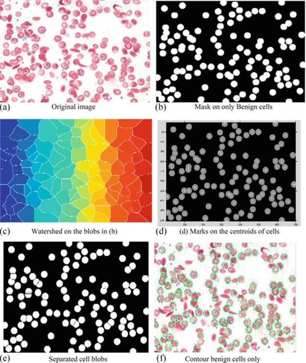
FIGURE 6 (a) The original image, (b) the healthy cells masked, (c) watershed for each blob region, (d) a small mark on each cell's centroid, (e) the cell blobs separated, and (f) the final detected benign cells.
In Figure 6(b), a mask of balls is constructed using centroids and radii for each cell, which have been previously determined. In this case, and after the masking process, many overlapping benign cells appeared as one big region according to the shape and size of the normal cells. For that reason, the watershed process in Figure 6(c) is applied to get the optimum separation in this abnormal shape of cells. In fact, to get the optimal separation of overlapped cells, their centroids are used to put marks on them as in Figure 6(d). Now the cells within each cell blob have been separated and marked, as in Figure 6(e). Finally, by applying all the previous steps, the benign cells are contoured by gray lines, extracted to count, and distinguished from the other distorted cells, which are also shown in the second step of part one. This detection operation indicates 109 benign cells out of 180 detected cells (benign and distorted) in the image. In fact, the remaining cells (71) may be considered to be detection errors, distorted cells (sickle-cell Anemia), platelets, or even WBCs. The image in the figure does not have any WBCs, but if WBCs exist in other images, the proposed algorithm can easily detect and count them, as in Figure 7. On the other hand, platelets have been neglected because the algorithm concentrates only on RBCs and those distorted cells that occur with sickle-cell anemia [21].
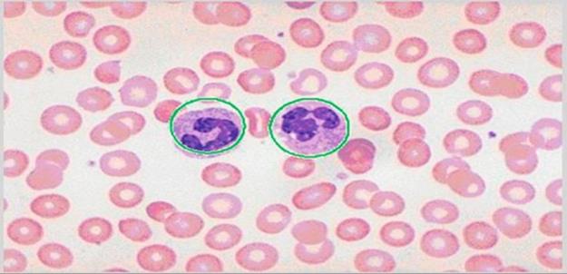
FIGURE 7 The detected WBCs.
Additionally, the algorithm has identified 177 cells, representing a 99.98% success ratio according to the image in Figure 6(a). Therefore, the next step is trying to discover how many of the 71 nonbenign cells are currently or potentially sickle cells. First, all 71 strange shapes (crescent, elliptic, platelets, and unknown) are discovered and displayed using the previous steps of benign cell detection. Figure 8 illustrates the last two steps of the proposed algorithm, which is applied to the distorted cells.
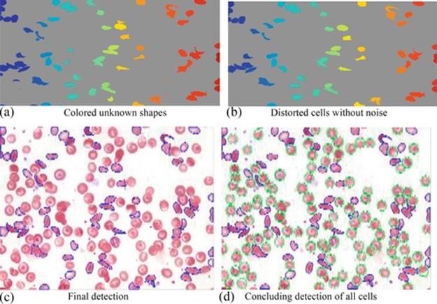
FIGURE 8 (a) All unknown shapes, (b) the distorted cells, (c) the final detection of only distorted cells, and (d) the final detection of all cells.
In Figure 8(a), a colored, segmented image shows all unknown distorted shapes with a noise similar to that produced by platelets, and so on. The current and potential sickle cells are detected without any noise in Figure 8(b). As a result, the deformed cells (current or potential sickle) appear to number 57 out of 71. The final detection of distorted cells is contoured by blue lines, as shown in Figure 8(c). In Figure 8(d), the final detection and tracking of all cells (benign by gray color and distorted with dark gray color) has been completed.
In this experiment, the NN consists of 4 input variables, 10 neurons in one hidden layer, and 1 output layer. The network succeeds after 65 of 1000 maximum iterations of the epoch, with a performance value of 0.0189, a gradient of 0.0165, and six validation checks, as shown in Figure 9(a). In Figure 9(b), the best validation performance is shown as 0.00010338 at epoch 59, with the training in a dark gray line, validation in a gray line, and the test in a red line. In the same context, the MSE of training, validation, and testing processes are 2.059e−2, 1.03383e−2, and 1.17910e−2, respectively.
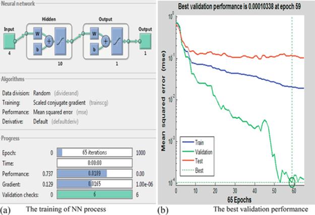
FIGURE 9 (a) The back-propagation NN, and (b) the best validation performance.
Figure 10 shows the confusion matrices for training, validation, and testing processes. In this figure, the predictions of the NN model are compared with the original classes of the target Tc to identify the values of TPs, TNs, FPs, and FNs. These values are computed to construct the confusion matrix, in which each cell contains the number of cases classified for the corresponding combination of desired and actual classifier outputs; it achieved 96.9%. Accordingly, accuracy, sensitivity, and specificity approximate the probability of the positive and negative labels being true and assess the usefulness the algorithm on an NN model. The accuracy, sensitivity, and specificity classifications of NN have achieved 98.4, 100, and 93.3% success with training samples, respectively.
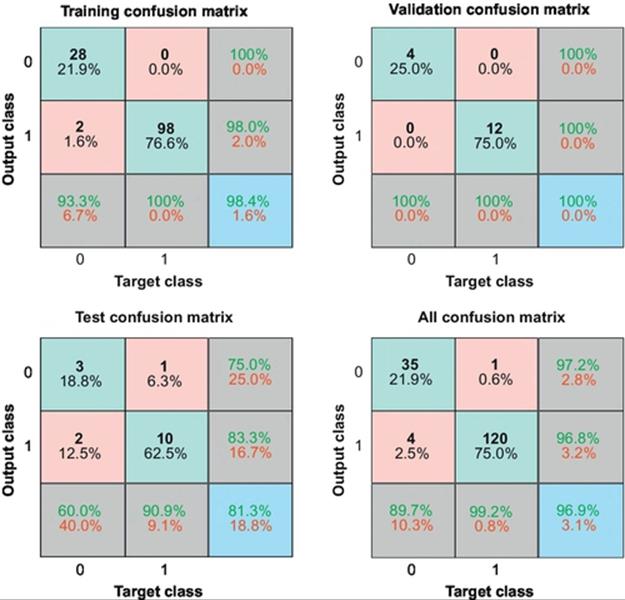
FIGURE 10 The confusion training, validation, and testing matrices.
Yet importantly, the NN agreed with the detection of cells using the proposed algorithm by about 96.9%.
Next, I apply the C&R tree to the mentioned input and target variables. The tree is carried out with a maximum depth of 5, a maximum of five surrogates, and the use of the Gini index to measure impurity. As in the previous example, the tree has trained 144 or 80% of all samples, and used 36 samples in validation and testing (i.e.. 20%). As a result, the tree achieved 95.83% agreed with the target in the training process, whereas, in the testing samples (cells), achieved 92.86% correct. Moreover, the most important and effective determined input variable is the eccentricity around 0.6786. The area variable comes in after eccentricity about 0.2576, followed by the perimeter variable around 0.0358 and the convex area variable at the end about 0.0279. Therefore, when using the C&R tree, the diagnosis may depend on the eccentricity, and, if necessary, the area variables, to distinguish the benign cells from the distorted ones.
Furthermore, the accuracy, sensitivity, and specificity in training samples have achieved 89.8%, 100%, and 82.1%, respectively. On the other hand, in the test samples, the accuracy, sensitivity, and specificity achieved approximately 81.25%, 100%, and 66.7%, respectively. Although the C&R tree is easier to apply to exported data than the NN is, it has achieved only about 92.9% success, while NN has achieved 96.9%. Clearly, the previous application of NN and C&R tree for the output data tends to show that NN is preferred and more effective than the C&R tree for making predictions from these data. In other words, the NN appears to be more effective at testing and checking the efficiency of the data resulting from the proposed algorithm in order to detect the sickle cells among all those distorted and, thus, to diagnose sickle-cell anemia. Finally, Matlab 2013a has been used to build the algorithm on Windows 7 with the processor Intel ® Core™2Duo CPU T5550@ 1.83 GHz, 2.50 GB RAM, and a 32-bit operating system. The optical Nikon microscope digitized all blood cell images.
8 Conclusions
The microscopic-image analysis of human blood cells is a valuable tool for detecting distorted blood cells. Sickle-cell anemia is one of the most important types of anemia. This chapter presents a proposed algorithm for detecting and counting the sickle cells among all healthy and distorted cells in a microscopic colored image, even if those cells are hidden or overlapped. I have used an algorithm with a CHT to detect benign and distorted blood cells. I then classified the exported variable data (e.g., area, convex area, eccentricity, and perimeter) for all detected cells (benign and distorted) as input variables, constructing a solidity measure for all cells as a target variable. In the next step, I applied the NN and regression tree to produce the right decision for diagnoses and to check the effectiveness of the proposed detection algorithm. Based on the experimental results, these procedures have demonstrated high accuracies, and these models appear successful at predicting the healthy and distorted cells present in blood from a person with sickle-cell anemia. I calculated the performance of the models, using three statistical measures: classification accuracy, sensitivity, and specificity. As a result, I have concluded that this algorithm has correctly segmented and classified about 99.98% of all input cells, which may have contributed to the improved diagnosis of sickle-cell anemia. The experimental results have shown that the effectiveness reaches to 96.9% in the case of applying an NN and 92.9% when using a C&R tree. Therefore, the proposed algorithm is very effective for detecting benign and distorted RBCs, and the NN is more efficient than a C&R tree for testing the quality of the detection algorithm.
References
[1] U. S. Department of Health & Human Services, National Institute of Health, 2014. http://www.nhlbi.nih.gov/.
[2] Image Processing Toolbox, is available through MATLAB's help menu, or online at: http://www.mathworks.com/help/images/index.html.
[3] Stockman GC, Agrawala AK. Equivalence of Hough curve detection to template matching. Commun ACM. 1977;20:820–822.
[4] Elsalamony HA, Elsayad AM. Bank direct marketing based on neural network. Int J Eng Adv Technol IJEAT. 2013;2(6):392 ISSN: 2249-8958.
[5] Breiman L, Friedman JH, Olshen RA, Stone CJ. Classification and regression trees. Belmont, CA: Wadsworth; 1998.
[6] Devi BR, Rao KN, Setty SP, Rao MN. Disaster prediction system using IBM SPSS data mining tool. Int J Eng Trends Technol (IJETT). 2013;4(8):3352 ISSN Volume: 2231.
[7] Hirimutugoda YM, Wijayarathna G. Image analysis system for detection of red cell disorders using artificial neural networks. Sri Lanka J Biomed Inform 2010;1(1):35–42.
[8] Das DK, Chakraborty C, Mitra B, Maiti AK, Ray AK. Quantitative microscopy approach for shape-based erythrocytes characterization in anaemia. J Microsc 2013;249(Pt 2):136–49. Received 7 August 2012; accepted 11 November 2012.
[9] Thirusittampalam K, Hossain MJ, Ghita O, Whelan PF. A novel framework for cellular tracking and mitosis detection in dense phase contrast microscopy images. IEEE J Biomed Health Informat. 2013;17(3):42–653.
[10] Khan HA, Maruf GM. Counting clustered cells using distance mapping. In: International conference on informatics, electronics & vision (ICIEV); 2013:1–6.
[11] Mushabe MC, Dendere R, Douglas TS. Automated detection of malaria in Giemsa-stained thin blood smears. In: 35th annual international conference of the IEEE engineering in medicine and biology society EMBC; 2013:3698–3701.
[12] Mukherjee R. Morphometric evaluation of preeclamptic placenta using light microscopic images. Biomed Res Int 2014;2014:9 pages. Article ID 293690.
[13] Fleyeh H, Biswas R, Davami E. Traffic sign detection based on AdaBoost color segmentation and SVM classification. In: EUROCON conference, IEEE, 1-4 July; 2013:2005–2010.
[14] Freeman WJ. The physiology of perception. Sci Am. 1991;264(2):78–85 University of California, Berkeley.
[15] Chaudhuri B, Bhattacharya U. Efficient training and improved performance of multilayer perceptron in pattern classification. Neurocomputing. 2000;34:1–27.
[16] Wikipedia, the free encyclopedia, (Redirected from Neural network), last modified 21 Oct 2014. http://en.wikipedia.org/wiki/Neural_network#History of the neural network analogy.
[17] YuBo T, XiaoQiu Z, RenJie Z. Design of waveguide matched load based on multilayer perceptron neural network. In: Proc ISAP, Niigata, Japan; 2007.
[18] Mitchell TM. Machine learning. New York: McGraw-Hill; 1997.
[19] Brown SD, Myles AJ. Decision tree modeling in classification. In: Brown SD, Tauler R, Walczak B, eds. Comprehensive chemometrics. Oxford: Elsevier; 2009:541–569.
[20] Atherton TJ, Kerbyson DJ. Size invariant circle detection. Image Viscion Comput. 1999;17(11):795–803.
[21] Elsalamony HA. Sickle anemia and distorted blood cells detection using Hough transform based on neural network and decision tree. In: Proc. international conference on image processing, computer, vision, and pattern recognition. IPCV’14, Worldcomp’14, Las Vegas, Nevada, USA; 2014:45–51.
All materials on the site are licensed Creative Commons Attribution-Sharealike 3.0 Unported CC BY-SA 3.0 & GNU Free Documentation License (GFDL)
If you are the copyright holder of any material contained on our site and intend to remove it, please contact our site administrator for approval.
© 2016-2026 All site design rights belong to S.Y.A.