Emerging Trends in Image Processing, Computer Vision, and Pattern Recognition, 1st Edition (2015)
Part III. Registration, Matching, and Pattern Recognition
Chapter 32. Surface registration by markers guided nonrigid iterative closest points algorithm
Dominik Spinczyk Faculty of Biomedical Engineering, Silesian University of Technology, Zabrze, Poland
Abstract
The problem of matching irregular surfaces was tested with additional markers as landmarks for the extension of the nonrigid iterative closest points algorithm. The general idea of presented approach was to take into account knowledge about markers' positions not only in computing transformation phase but also in finding correspondence phase in every algorithm's iteration. Four variants of retrieving correspondence were implemented and compared: the Euclidean distance, normal vectors with initial rigid registration, static and dynamic markers vectors. To evaluate different manner of computing correspondence the average correspondence assignment error of points nearest to the markers and the number of correspondences for every target points were defined. The presented approach was evaluated using abdominal surfaces data set consisting of captured clouds of points during free breathing of six volunteers. The modifications significantly improved results. To make the proposed changes more universal k-nearest neighbor method and radius constraint could be used.
Keywords
Markers guided geometry-based registration
Finding correspondences
Nonrigid iterative closest points
Surface registration quality
Surface registration
Acknowledgment
The study was supported by National Science Center, Poland, Grant No UMO-2-12/05/B/ST7/02136.
1 Introduction
Registration is a process to find correspondence between data sets, and generally could be divided into geometry-based or intensity-based methods [1]. Nowadays, in many multimedia applications input data set are represented as point cloud (segmented surfaces of the objects, etc.). Then in the processing pipeline data sets should be register, to find the correspondence between data sets. The most popular approach, in this case, is iterative closest point algorithm (ICP) [2]. This algorithm was proposed by a few researchers independently [3,4]. The ICP is an iterative algorithm and consists of two steps. The first step is to find a correspondence between target and source points, based on Euclidean distance between points. In the second step, the updated version of result transformation is calculated using equation:
 (1)
(1)
where T, S are target and source set of points, Ns is number of source points (equals number of target points), and Rot, Trans are rotation and translation components of final transformation.
The updated version of final transformation in current iteration is based on close-form solution of mean square error problem. The classical approach used only one rigid or affine transformation for whole data sets. In literature the description of disadvantages of the classical ICP approach [5] can be found:
• problem of finding global minimum of cost function depends on an initial guess of final transformation,
• the algorithm is sensitive to improper correspondences,
• long time of computation—one of the most time-consuming operation is retrieving correspondences.
Due to these disadvantages researchers proposed a lot of classical approach rectifications:
• registration only subsets of points,
• improvement of finding correspondence problem,
• quantity measure of proper correspondence,
• elimination of improper correspondence,
• modification of computing minimum of cost function.
The standard ICP approach cannot be used to track surface of objects that change their shape in time. Amberg [6] proposed nonrigid version of ICP by the following equation:
![]() (2)
(2)
where X is the unknowns organized in a 4n × 3 transformation matrix; Ed(X) is distance measure between all target points and transformed source points, in contrast to classical ICP. X is not a single rotation or translation but a collection of affine transformation for each point; Es(X) is stiffness regularization, topology matrix is created based on points neighborhood to preserve the shape of object during iterations; we use square matrix topology (every point has four neighbors). α is stiffness vector, which influences the flexibility of cloud shape; βE1(X) is a factor used for guiding registration, based on known position of landmarks in source and target sets of points. β is a weighting factor, used to fade out the importance of landmarks toward the end of the registration process.
The implemented nonrigid ICP algorithm consists of two iterative loops. In the outer loop, the stiffness factor α is gradually decreased with uniform steps, starting from higher values, which enables recovery of an initial rigid global alignment, to lower values, allowing for more localized deformations. For a given value of α, the problem is solved iteratively in the inner loop. The condition of changing stiffness vector is threshold norm of transformation difference from adjoining iterations. In our implementation β is constant and equals 1. The above equation can be transformed into the system of linear equations, which is solved by computing pseudo-inverse matrix (see Amberg et al. [6] for details). This is the iterative algorithm, where each iteration consists of two main steps, namely finding correspondences between source and target points and computing affine transformations for each source point. If the second step is modified by the solution proposed by Amberg, that causes better results, corresponding problem remains critical for final results.
2 Materials and methods
Improvement of finding correspondences was implemented. Classically finding correspondences are done by searching Euclidean distance between closest points in source and target or in normal vector of source point direction. The general idea of presented approach was to take into account knowledge about markers' positions not only in computing transformation phase but also in finding correspondence phase in every algorithm's iteration. Decision to test a few approaches of finding correspondences was done:
• searching along normal vectors in source points, following the initial rigid registration based on Horn algorithm [7],
• along static marker vector displacement, where marker vectors are calculated only once at the preliminary stage. Marker vector is defined by positions of specific marker in source and target point cloud,
• along dynamic marker vector displacement, where marker vectors are calculated in each iteration based on constant positions of nearest marker points in matrix topology. Transformed source point in each iteration is treated as a new origin of dynamic marker vector.
Classical Euclidean distance is treated as baseline to compare the obtained results. Generally it is challenging to verify registration approach. We used global and local criteria for evaluation:
• global measurement: average distances between nearest source and target points, average distances between correspondences,
• local measurement—quality of correspondences: average correspondence assignment error of points nearest to the markers and the number of correspondences for every target points.
Data set consists of abdomen surfaces acquired by six volunteers on free breathing using time-of-flight sensor Mesa SR4000 [8]. Intensity map example of input data is presented in Figure 1. As markers 15 mm white squares attached to the abdomen were used, which corners were manually segmented by two users.
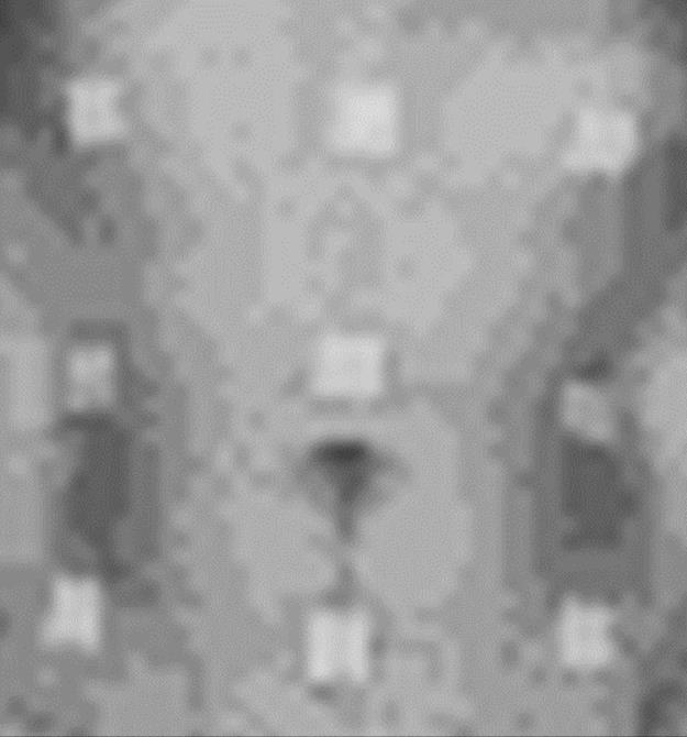
FIGURE 1 Example of input data: intensity map for ToF camera of abdomen with nine square markers.
3 Results
For the different methods of finding correspondences, evaluation scores: surface distances, correspondence distances and average marker error, are presented in Tables 1 and 2.
Table 1
Surface distances for four variants of ICP
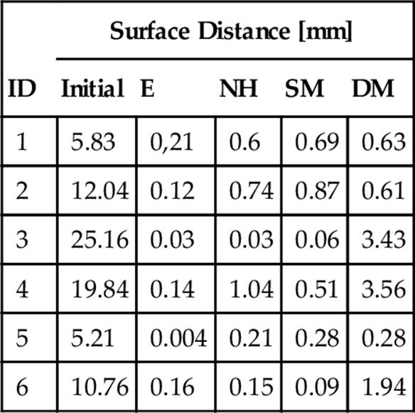
E, the Euclidean distance; NH, normal vectors with initial rigid registration; SM, static; DM, dynamic markers vectors.
Table 2
Correspondence distances and average marker error for four variants of ICP
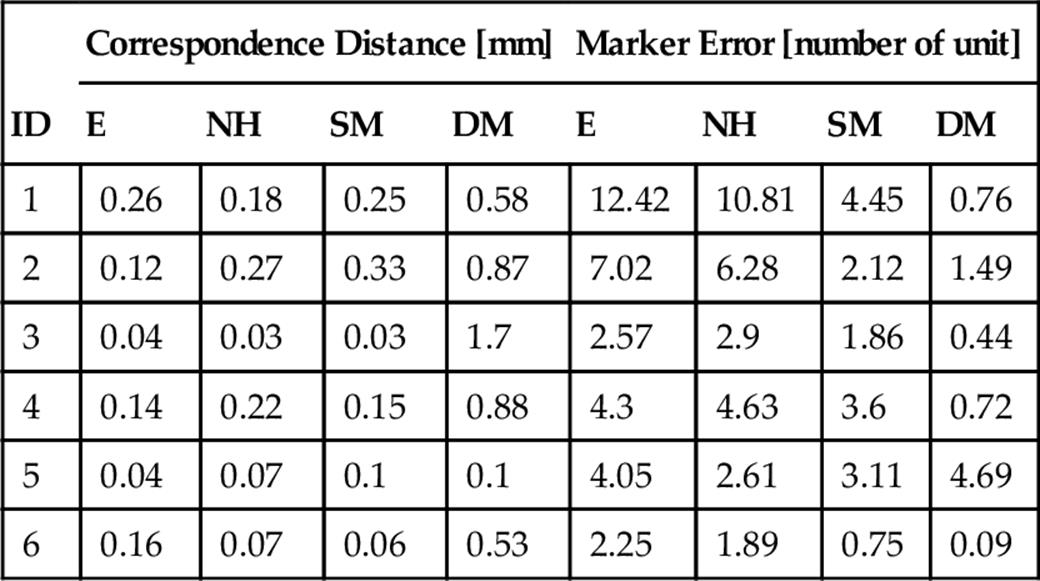
E, the Euclidean distance; NH, normal vectors with initial rigid registration; SM, static; DM, dynamic markers vectors.
4 Discussion and conclusions
The implemented nonrigid ICP algorithm showed average residual distance of 0.68 mm (Euclidean distance not included). A further analysis of registration accuracy was focused on finding correspondence problem. Four methods for this problem were tested: Euclidean distance treated as base line, normal shooting with initial rigid registration—marker-based Horn algorithm, static marker vectors (computing only one at the beginning of registration process), and dynamic marker vectors (computing in every iteration). For “near” cloud, where stiffness vector is constant for almost every iterations in nonrigid ICP, Euclidean distance is good enough. Unlike “near” clouds, “far” clouds, where stiffness vectors are changing for few iterations, Euclidean distance seems to be not enough. There are a lot of gaps in registered source cloud (Figure 2). To improve it, static and dynamic marker vectors were proposed. If marker is not only used in computing transformation step but also in computing correspondences step for each iteration, correspondence assignment error of points nearest to the markers decreased from 5.4 to 2.0 of confused neighbors. Normal shooting approach was also evaluated, but results were worse than other cases, while combination normal shooting and initial rigid registration significantly improved results (Figure 2). To use Horn algorithm at least three noncollinear corresponding points in source and target should be known. It helps to overcome the problem of the relative displacement of the source and target point clouds, which is not taking into account when Euclidean distance is used.
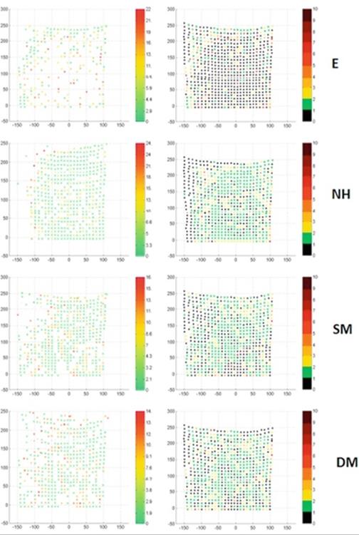
FIGURE 2 Distance map [mm] (left column) and correspondence map [number of units] (right column) for different modifications of ICP computing correspondence: Euclidean distance (E), normal shooting with initial rigid registration (NH), static marker vectors (SM), and dynamic marker vectors (DM).
Because it is difficult to measure directly the quality of correspondences, observation was proposed in a few steps. Correspondence map (Figure 2) showed spatial distribution of the feature, number of correspondences assigned to every target point (desirable value is 1). It is easier to compare correspondence map globally with different cases using correspondence map histogram (Figure 3). Average correspondence assignment error of points nearest to the markers allows to measure the quality of correspondence points from cloud, which are nearest to the markers.
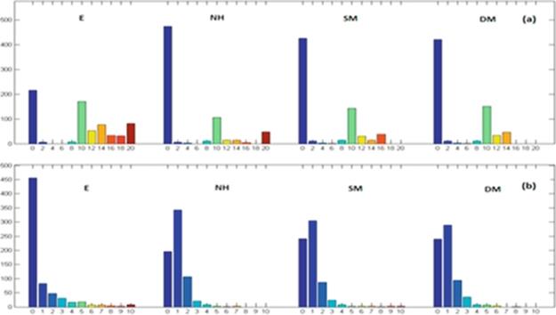
FIGURE 3 Distance map histogram [mm] (a) and correspondence map histogram [number of units], (b) in different modifications of ICP computing correspondence: Euclidean distance (E), normal shooting with initial rigid registration (NH), static marker vectors (SM), and dynamic marker vectors (DM).
The results show improvement when markers are used not only in computing transformation phase but also in finding correspondence phase in every algorithm's iteration [9]. To make the proposed changes more universal k-nearest neighbor method and radius constraint could be used to apply the marker information to not only every point in the cloud but also the nearest points to the markers. For points that are not near a marker, the Euclidean distance was used. The score results for three selected values (i.e., 5, 10, and 15%) of the radius constraint selected as percent of the cloud width were calculated. The results are presented in Figure 4. For the most demanding criterion (5%), the results showed improvement.
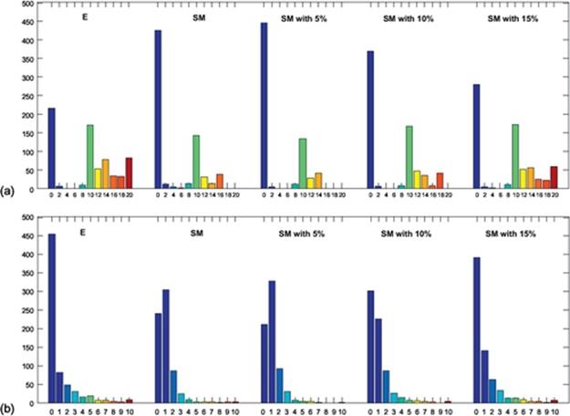
FIGURE 4 Distance map histogram [mm] (a) and correspondence map histogram [number of units], (b) for different modifications of the ICP computing correspondence algorithm: static marker vector (SM) and static marker vector with 5, 10, and 15% radius constraints for the ToF camera.
The convergence of ICP algorithm is topic of research [10]. In presented approach no reliability weighting is used (weighting is always equal 1), the residual in an optimal step ICP is always decreased, because neither finding a new deformation, nor finding new closest points can increase residual. A formal proof for rigid case, which can be applied to presented approach can be found in Ref. [2]. Danilchenko and Fitzpatrick [11] proposed principal access approach to taking into account local character of anisotropic noise in rigid point registration and Maier-Hein et al. [10] used this approach to rigid anisotropic weighting ICP algorithm and ToF data. In future work this approach can be generalized to nonrigid ICP.
Presented approach may be used in different medical, entertainment, and industrial applications, where nonrigid point clouds should be registered, when initial relative position of clouds is that finding correspondences by Euclidean distance or normal shouting is not enough. The proposed changes do not introduce complex calculations. Initial calculation of rigid registration allows to solve the problem of unknown transformation matrix initialization. Comparing to classical nonrigid ICP the disadvantage of proposed approach is that initial corresponding positions of markers in source and target point clouds are needed.
References
[1] Wyawahare M, Patil P, Abhyankar H. Image registration techniques: an overview. Int J Signal Proc Image Process Pattern Recogn. 2009;2(3):11–28.
[2] Salvia J, Mataboscha C, Fofib D, Forest J. A review of recent range image registration methods with accuracy evaluation. Image Vision Comput. 2007;25:578–596.
[3] Besl P, McKay N. A method for registration of 3D shapes. Pattern Anal Mach Intell. 1992;14(2):239–256.
[4] Chen Y, Medioni G. Object modeling by registration of multiple range images. Image Vision Comput. 1992;10(3):145–155.
[5] Rusinkiewicz S, Levoy M. Efficient variants of the ICP algorithm. In: Proc. 3rd international conference on 3D digital imaging and modeling; Stanford, CA: Stanford University; 2001:145–152.
[6] Amberg B, Romdhani S, Vetter T. Optimal step nonrigid ICP algorithms for surface registration. In: Proc. IEEE conference of computer vision and pattern recognition CVPR; 2007:1–8.
[7] Horn B, Hilden H, Negahdaripour S. Closed form solution of absolute orientation using orthonormal matrices. J Opt Soc Am A. 1988;5:1127–1135.
[8] http://www.mesa-imaging.ch/swissranger4000.php – Mesa-Imaging – manufactor website: SR4000 Data Sheet.
[9] Spinczyk D (2014). Surface registration by markers guided non-rigid iterative closest points algorithm. Proc. 2014 international conference on image processing, computer vision, and pattern recognition.
[10] Meier-Hein L, Franz A, Santos T, Schmidt M, Fangerau M, Meinzer H, et al. Convergent iterative closest-point algorithm to accommodate anisotropic and inhomogenous localization error. IEEE T Pattern Anal Mach Intell. 2012;34(8):1520–1532.
[11] Danilchenki A, Fitzpatrick J. General approach to first-order error prediction in rigid point registration. IEEE Trans Med Imaging. 2011;30(3):679–693.
All materials on the site are licensed Creative Commons Attribution-Sharealike 3.0 Unported CC BY-SA 3.0 & GNU Free Documentation License (GFDL)
If you are the copyright holder of any material contained on our site and intend to remove it, please contact our site administrator for approval.
© 2016-2026 All site design rights belong to S.Y.A.