Emerging Trends in Image Processing, Computer Vision, and Pattern Recognition, 1st Edition (2015)

Part III. Registration, Matching, and Pattern Recognition

Chapter 33. An affine shape constraint for geometric active contours

Mohamed Amine Mezghich; Maweheb Saidani; Slim M’Hiri; Faouzi Ghorbel GRIFT Research Group, CRISTAL Laboratory, Ecole Nationale des Sciences de l’Informatique (ENSI), Campus Universitaire de la Manouba, Manouba, Tunisia

Abstract

In this paper we intend to present an original approach that incorporates shape prior into a geometric active contours. A Fourier-based shape alignment method is used to define prior knowledge from a given reference shape. At a first step, we propose an invariant shape prior with respect to some Euclidean transformations (translation, rotation, and scaling factor). Then, we generalize to the case of affine ones. In order to take into account the multireferences situation, we present a set of complete and stable invariant shape descriptors computed using Fourier transform of the contours to choose the most suitable reference according to the evolving contour. To balance the strength between the image-derived force and the proposed shape prior force, a weighting schema is introduced to guide the model evolution under both forces. Experimental results show the ability of the new added term to constrain an evolving curve meet target shape and show the new method benefits on segmentation results in presence of occlusion, clutter, and noise.

Keywords

Active contours

Shape prior

Contours alignment

Fourier transform

Motion estimation

1 Introduction

Precise object of interest detection is of high need in many applications of image processing such as medical imaging, tracking of moving object, and 3D object reconstruction. There have been several works in this field of image segmentation and object detection. Among them we can distinguish the classical active contours which are intensity-based models [1–5] and the constrained models by a prior knowledge that are driven both by global geometrical [6–9] or statistical [10–14] shape information and a local image information like gradient or curvature. There have been promising results given that the classical snake models can detect object with smooth contours whereas the level set-based models have the additional ability to detect simultaneously many objects in the image. However, several work of the prior knowledge-driven models reached good segmentation results by detecting partially occluded shapes presenting missing part in low contrast or very noisy image. To define prior knowledge, the authors use either shape alignment [7] or registration [9] between the contour of the target shape and the shape of reference or a distance between invariant shape descriptors like [8]. All these work manage the case of Euclidean transformations (translation, rotation, and scale factor). But in real situations, the object of interest can submit large transformations (affine or projective cases) and distortions. Hence the class of rigid transformations is not appropriate to model this type of movement between the shape of reference and the target one. To our knowledge, there has been only the work of Foulonneau et al. [15] that treats the case of affine transformations. Although this approach, which is based on the distance between an invariant set of Legendre descriptors of the target and reference shapes, presented good results, this method suffers from the instability of the Legendre moments and the order that has to be fixed empirically. Besides, the method requires a heavy execution time to achieve satisfactory results. In order to extend the work of shape priors presented in Refs. [16,17], we propose in this research a geometric approach to manage the class of affine transformations [26] that can occur between the shape of interest and the reference one. Prior knowledge is obtained by aligning the evolving contour and the template using an alignment method which is based on Fourier descriptors. For this purpose, we will start by introducing our approach in the case of rigid transformations. Then we generalize the idea by treating the case of affine ones that often occur in real situations. We will also propose a geometric method based on a set of complete and stable set of invariant shape descriptors to manage the case of mutireferences. Combining the proposed shape prior information with the level set-based model, the improved model can retain all the advantages of the active contour model and have the additional ability of being able to represent the global shape of an object. The remainder of this paper is organized as follows: In Section 2, a description of the outlines of the used shape alignment method in both cases (Euclidean and affine transformations) will be presented. In Section 3, we will briefly recall the principle of the used edge-based active contours, then we will move to present the proposed shape prior. Experimental results are presented and commented in Section 4. Finally, we conclude the work and highlight some possible perspectives in Section 5.

2 Shape alignment using fourier descriptors

In this section, we recall the used alignment methods to define the proposed energy in both cases rigid and affine transformations.

2.1 Euclidean Shapes Alignment

It is well known that the closed contour of a planar object can be given by its parametric representation

(1)

Let γ₁and γ₂ be centered (according to the center of mass) and normalized arc length parameterizations of two closed planar curves having shapes F₁and F₂. Suppose that γ₁ and γ₂ have a similar shape under rigid transformation.

In shape space this is equivalent to have:

(2)

where α is the scaling factor, θ the rotation angle, t₀ is the difference between the two starting points of γ₁ and γ₂.

Rigid motion estimation is obtained by minimizing the following quantity introduced by [18]:

(3)

If αis equals to 1 [19], showed that Equation (3) is a metric in shape space and corresponds to the Hausdorff distance between the two shapes. In practice, this result implies the uniqueness of the motion's parameters so obtained. Using Fourier descriptors C_k(γ₁) and C_k(γ₂), minimizing E_rr becomes equivalent to minimize f(θ, t₀) in Fourier domain

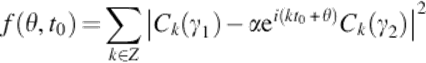(4)

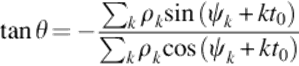
[18] proposed an analytical solution to compute t₀ and θ. t₀ is one of the zeros of the following function:

(5)

where , θ is chosen to satisfy Equation (6) and minimize f(θ, t₀) where t₀ is one of the roots of Equation (5).

(6)

Having the value of θ and t₀ that minimize f(θ, t₀), the scaling factor is given by

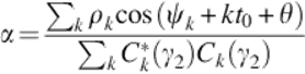(7)

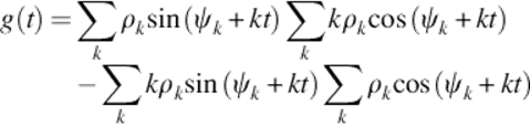
Based on Nyquist-Shannon theorem and B-spline approximation of the g(t)'s curve, Persoon and Fu [19] proposed the first implementation of this method of shape alignment and its application in rigid motion estimation for video compression. In Figure 1, we give an example of two aligned curves with the used method.

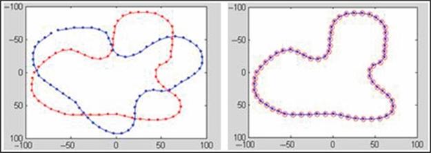
FIGURE 1 Example of two curves before (a) and after (b) shape alignment.

The estimated motion's parameters are presented in Table 1. The associated g(t)'s curve is presented in Figure 2. The zeros of g(t) are drawn with circles.

Table 1

The Estimated Parameters of Synthetic Rigid Motion

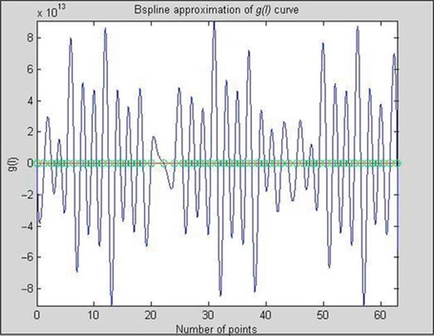
FIGURE 2 Example g(l)'s curve.

2.2 Affine Shape Alignment

In order to define affine invariant shape prior from a reference shape, we have to perform shape matching between the target and the template shapes F₁ and F₂. To correctly estimate the affine motion parameters, we have to deal with the same number of points which is not relevant if we consider two different points of view. For this purpose, in Ref. [20], the author proposes to use the affine reparametrization of curve which is invariant under affine transformation. We will start by presenting the affine reparametrization procedure of a given curve. Then we will describe our method of affine motion's parameters estimation.

2.2.1 Reparametrization of closed curve

If we take the same object in two different camera sides, we found a different number of contour points in each image. Consequently, we proceed by normalization of curves under affine transformation. Given the shape front, its edge pixels are extracted and traversed to yield a discrete closed curve which is a parametric equation γ(t) = (u(t), v(t)), where t ∈ {0,…,N − 1} and γ(N) = γ(0). We use the affine arc length reparametrization to normalize closed curves under affine transformations that can be expressed by:

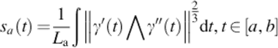(8)

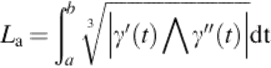(9)

where L_a is the total affine arc length of the considered curve, ∧ represents the cross product between two vectors and, ||·|| denotes the Euclidean norm.

2.2.2 Contours alignment using geometrical affine parameters estimation

We consider two closed curves O₁and O₂which define the same shape. O₁and O₂ are said to be related by an affine transformation if and only if:

(10)

where Bis a translation vector, A is a linear transformation, l₀ is the shift value, f and h are the affine reparametrization of two contours having the same affine shape. In the Fourier space we get:

(11)

where U_k(h) and U_k(f) are, respectively, the Fourier coefficients of f and h.

So estimation of affine motion can be resumed to the estimation of its three parameters: the affine matrix A, the shift value l₀, and finally the scale factor α if we consider a normalization under translation.

Estimation of the scale factor α

The scale factor can be estimated using the following formula:

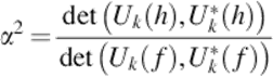(12)

where and are 2 × 2 matrix formed by Fourier coefficients on some fixed index k and U* is the U complex conjugate.

Computation of the shift value l₀

Let's consider and

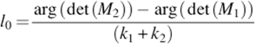(13)

where k₁ and k₂ are two fixed index and arg(U) is the complex argument of U.

Computation of the matrix A's parameters

Since scale factor α and shift value l₀have been previously estimated (Equations 12 and 13), we are going to estimate affine matrix A parameters. Lets O₁, O₂ be two curves and U_f, U_h, respectively, their Fourier coefficients. In Fourier space we have (Equation 14)

(14)

Using matrix, we have the following formula:

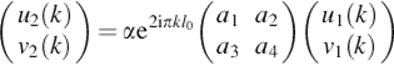(15)

So we have to estimate a₁, a₂, a₃, and a₄. This system can be represented as following:

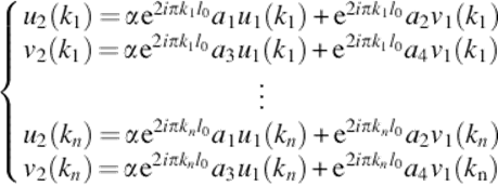(16)

Then to estimate matrix A's parameters (Equation 14), we have to resolve a system with 2N equations and four unknown parameters that can be written as

(17)

The solution of the system (Equation 16) can be obtained by

(18)

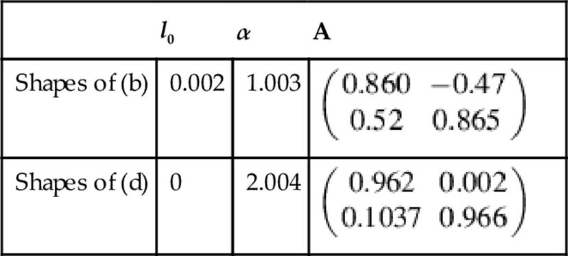
So we have to minimize the quadratic error e by using the pseudoinverse of K. We show by the following figure an example of affine motion estimation between two synthetic curves after contours resampling (Figure 3). The final result of curves alignment after affine motion estimation is presented by Figure 4. The estimated motion parameters are presented in Table 2.

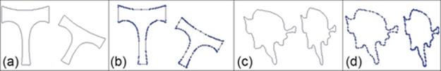
FIGURE 3 Two different shapes after affine deformations ((a) and (c)) and curve resampling ((b) and (d)).

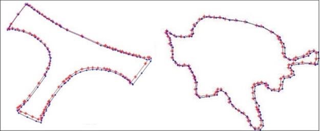
FIGURE 4 Results of affine shape alignment.

Table 2

The Estimated Affine Motion Parameters

2.3 Discussion

Having the parameters of the affine or Euclidean transformations between the two contours, we perform the alignment of the two curves to determine the regions of variability between shapes by computing the product function of the signed distance functions associated to level set functions of, respectively, the target and the reference object after alignment given by

(19)

where and f_∅ are the two binary images associated, respectively, to ∅ _ref and ∅. See Ref. [16] for more details. By construction, the product function f_prod is negative in the areas of variability between the two binary images and f_∅ due to occlusion, clutter, or missing parts, whereas in positive regions, the objects are similar. Thus, in what follows, we propose to update the level set function ∅, only in regions of variability between shapes to make the evolving contours overpass the spurious edges and recover the desired shapes of objects. This property recalls the narrow band technique used to accelerate the evolution of the level set functions [4].

2.4 Global Matching Using Affine Invariants Descriptors

In presence of many templates, we have to choose the most suitable one according to the evolving curve. Let αand β be positive real numbers, and k₀, k₁, k₂, and k₃ four positive integers.

Let C_n^x and C_n^y be the complex Fourier coefficients of the coordinates (u, v). Δ denotes the determinant.

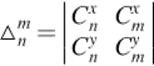(20)

In Ref. [20], the author introduced two sets of invariant descriptors I and J which are, respectively, given by (Equations 21 and 22).

(21)

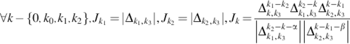(22)

In Refs. [21,22], the authors have shown experimentally that such descriptors are complete and stable. The completeness guarantees the uniqueness of matching. The stability gives robustness under nonlinear shape distortions and numerical errors. In Ref. [20], the author demonstrates that the shape space S can be considered as a metric space with a set of metrics. Hence, the Euclidean distance (Equation 23) between the set of the presented invariants can be used to compare the evolving curve and the available templates.

(23)

For any real number p such that p > 1. Where f and hare two normalized affine arc length reparametrization of two objects having, respectively, the shapes F and H. The shape having the minimum distance according to the evolving active contour is used as template.

3 Shape Prior for Geometric Active Contours

Geometric active contours are iterative segmentation methods which use the level set approach [2] to determine the evolving front at each iteration. Several models have been proposed in literature that we can classify into edge-based or region-based active contours.

In Ref. [4], the level set approach is used to model the shape of objects using an evolving front. The evolution's equation of the level set function ∅ is

(24)

F is a speed function of the form F = F₀ + F₁(K) where F₀ is a constant advection term equals to (± 1) depends of the object inside or outside the initial contour. The second term is of the form − εK where K is the curvature at any point and ε > 0. To detect the objects in the image, the authors proposed to use the following function which stops the level set function's evolution at the object boundaries.

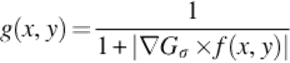(25)

where f is the image and G_σis a Gaussian filter with a deviation equals to σ. This stopping function has values that are closer to zero in regions of high image gradient and values that are closer to unity in regions with relatively constant intensity. Hence, the discrete evolution equation is:

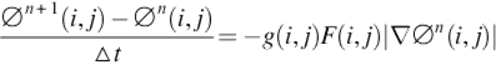(26)

It's obvious that the evolution is based on the stopping function g which depends on the image gradient. That's why this model leads to unsatisfactory results in presence of occlusions, low contrast, and even noise. To make the level set function evolve in the regions of variability between the shape of reference and the target shape, we propose the new stopping function as follows:

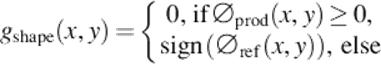(27)

where ∅ _prod(x, y) = ∅ (x, y) ∙ ∅ _ref(x, y), ∅ is the level set function associated to the evolving contour, while ∅ _ref is the level set function associated to the shape of reference after alignment. As it can be seen, the new proposed stopping function only allows for updating the level set function in the regions of variability between shapes. In these regions, g_shapeis either 1 or − 1 because in the case of partial occlusions, the function is equal to 1 in order to push the edge inward (deflate) and in case of missing parts, this function is equal to − 1 to push the contour toward the outside (inflate). This property recalls the Balloon snake's model proposed by Cohen [23] in which the direction of evolution (inflate or deflate) should be precise from the beginning. In our work, the direction of evolution is handled automatically based on the sign of ∅ _ref. The total discrete evolution's equation that we propose is as follows:

(28)

w is a weighting factor between the image-based force and knowledge-driven force. See Ref. [16] for our proposed shape prior for a region-based active contours.

4 Experimental results

4.1 Robustness of the Proposed Shape Priors

We present in Figure 5 an example of successive evolutions between several shapes of different topologies under the proposed shape priors only (w = 0). By the first row, the initial shape is a simple square while the target is a tree leaf. For the second row, the final shape obtained after several iterations in the first row is used as initial contour. The template in this case consists of two contours. This experiment proves that the proposed shape constraint can act on the topology of the original curve. Finally, by the third row, we show the ability of our shape prior to detect objects with holes.

FIGURE 5 Curve evolution under the proposed shape prior only.

This simulation shows that the proposed shape priors can well constrain an active contour to take a given shape (known as reference) and handling nontrivial geometric shapes with holes and complex topologies.

4.2 Application to Object Detection

We will devote this section to present some satisfactory results obtained by the proposed model in the case of Euclidean transformations, then the general case of the affine ones will be treated. The algorithm is as follows: We first evolve the active contour without shape prior until convergence (i.e., w = 1) to reduce the computational complexity and to have a good estimation of the parameters of the geometric transformation as in Refs. [8,11]. This first result provides an initialization for the model with prior knowledge. Then the model will evolve under both forces (data and prior forces) with more weight assigned to prior knowledge (generally w ≤ 0.5) to promote convergence toward the target shape.

4.2.1 Case of Euclidean transformation

To assess the performance of the method, we have experimented the proposed method in medical imaging. The template is given by image 1 of Figure 6 which corresponds to the left ventricle of the heart. The aim is to detect the true contours of the left ventricle of the heart which are partially occluded by the valve. The second row of Figure 6 shows several iterations of curve evolution until convergence without prior knowledge. Starting with final this result, and based on the reference shape after rigid motion estimation, the evolving front continues its evolution until the curve reaches the desired contours (third row).

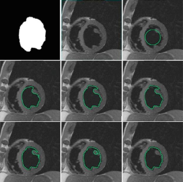
FIGURE 6 First row: The template, test image, initial curve. Second row: The active contours without shape prior. Third row: The active contours with shape prior.

The aligned curves which are used to compute the prior energy are presented in Figure 7. We present by Table 3, the estimated rigid motion parameters.

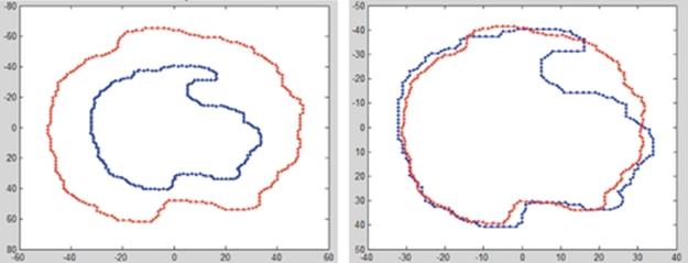
FIGURE 7 First image: Curves before alignment, Second image: Curves after alignment.

Table 3

The Estimated Motion's Parameters

We end this part of experiments by applying the active contour with shape prior to object tracking. In Figure 8, the goal is to track the mouse in a video sequence with cluttered background. We suppose that the movement of the mouse through frames is rigid thus the presented method of shape alignment is used. The convergent contour in frame i is used as a template in frame i + 1.

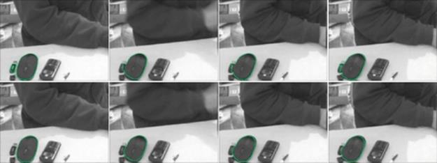
FIGURE 8 Tracking of the mouse in video sequence. First row: The active contours model without shape prior. Second row: The active contours model with shape prior.

Results seem to be satisfactory. Although, the presented rigid motion estimation method solves some situations and leads to interesting detection results. Other types of transformations such as stretching can only be solved by the class of relevant transformations. Thus the goal of the next section is to present some obtained results within this framework.

4.2.2 Case of affine transformation

Consider for this first experiment, the spider object, image (a) of Figure 9, obtained from MCD database (url: http://vision.ece.ucsb.edu/zuliani/Research/MCD/MCD.shtml). The (b) image is the object of interest which is obtained from (a) after affine transformation and partial occlusion. As a first step, we perform object (b) segmentation without prior knowledge. The obtained contour is then aligned with the contour of the (a) object to determine the regions of occlusions. We present in (c) the result of shape alignment. The estimated values are α = 2, l₀ = 0, A = [0.5, 0.2, 0, 2]. By Figure 10, we present the obtained results without and with shape prior. We considered in this experiment four templates (a spider, a chopper, a device, and a bird), see Figure 11. We were based on the set of the presented invariant shape descriptors to choose the suitable reference according to the occluded spider (image (b) of Figure 11).

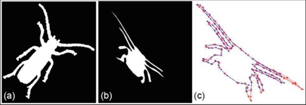
FIGURE 9 Spider's shapes alignment.

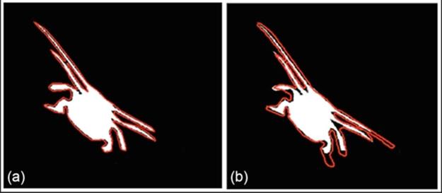
FIGURE 10 Detection without, image (a), and with, image (b), affine prior knowledge.

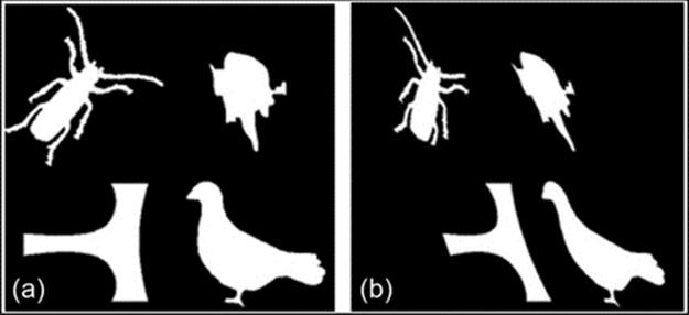
FIGURE 11 Image (a): The available templates. Image (b): The transformed object.

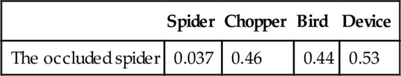
Table 4 presents the obtained Euclidean distance between the target shape and the available templates. We notice that the minimum distance can be easily identified because the suitable form in this experiment is distinguishable.

Table 4

Distances Between the Occluded Spider and the Used Templates

In the next experiment, a mosaic application is considered. The mosaic images that are considered are taken from the Bardo Museum of Tunisia which contains the biggest collection of mosaic images in the world. In mosaic images, objects are composed of tessellas and are often partially occluded as they are shown by images (c) and (d) (Figure 12).

FIGURE 12 Some mosaic images from the Bardo Museum of Tunisia.

So, given that in mosaic images the objects are often repeated and in order to study the robustness of our method, we try to find to true contour of an occluded object based on another one having the same shape. We have approximated the perspective projection to an affine transformation which is often used in the literature according to the acquisition conditions. Let's consider the (c) image. As it's shown, this image contains many forms. Among all forms available in these two images, (c) and (d), taken from two sides, we use the Euclidean distance between the affine invariant Fourier descriptors to localize two lions. The left one is partially occluded. We will use the right lion of the (d) image as template in order to have a better segmentation. In the last figure, images (a) and (b), we present the used curves to perform shape alignment and shape prior computation. The estimated values are α = 1, l₀ = − 0.52, A = [− 0.002, − 0.003, 2.003, − 0.35]. We present by the (c) image the obtained curves alignment result and by the (d) image the segmentation result based on the proposed shape prior. Such results are particularly interesting since it can be used for mosaic images restoration under partial occlusions and missing parts. The underlying idea is to extract similar forms using minimal distance between descriptors in order to define prior knowledge for such occluded or cluttered objects based on the presented affine shape alignment method for the purpose of a good segmentation result (Figure 13).

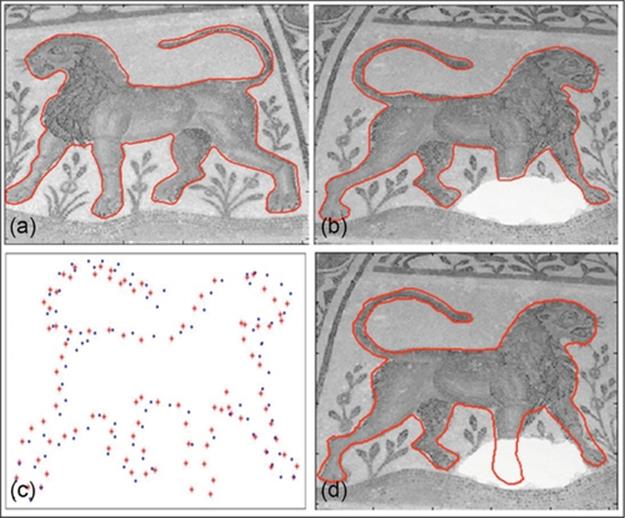
FIGURE 13 Robust object detection in mosaic image.

5 Conclusions

We presented in this paper an alternative approach to incorporate prior knowledge into a level set-based active contours in order to have robust object detection in case of large shape distortion that can be analyzed by the class of affine transformations. We presented also a geometric solution to choose the reference shape in case of many available templates, given that the statistical approach needs a training set and PCA. Then the application of a given classifier like Bayesian classifier to determine the appropriate reference shape like the work of Fang and Chan [24]. Given that the proposed approach invokes only pixels of the regions of variability between the shape of reference and the object of interest in the process of curve evolution and based on the fast Fourier transform for affine motion estimation and invariants computation, the method is faster compared to Refs. [15,25] where at each iteration shape descriptors are calculated for a given order that has to be set empirically. The obtained results are promising in the case of real and simulated data and the method can be used for the restoration of mosaic images in the archeological field. As future perspectives, we are working on integrating our model in the context of 3D object reconstruction from silhouettes sequence in order to refine the obtained 3D model.

References

[1] Kass M, Witkin A, Terzopoulos D. Snakes: active contour models. Int J Comput Vis. 1988;1:321–331.

[2] Osher S, Sethian JA. Fronts propagating with curvature-dependent speed: algorithms based on Hamilton-Jacobi formulation. J Comput Phys. 1988;79:12–49.

[3] Caselles V, Kimmel R, Sapiro G. Geodesic active contours. Int J Comput Vis. 1997;22:61–79.

[4] Malladi R, Sethian J, Vemuri B. Shape modeling with front propagation: a level set approach. PAMI. 1995;17:158–175.

[5] Chan T, Vese L. Active contours without edges. IEEE Trans Imag Process. 2001;10:266–277.

[6] Charmi MA, Mezghich MA, M’Hiri S, Derrode S, Ghorbel F. Geometric shape prior to region-based active contours using Fourier-based shape alignment. In: IEEE international conference on imaging systems and techniques; 2010:478–481.

[7] Charmi MA, Derrode S, Ghorbel F. Using Fourier-based shape alignment to add geometric prior to snakes. In: International conference on acoustics, speech and signal processing; 2009:1209–1212.

[8] Foulonneau A, Charbonnier P, Heitz F. Contraintes géométriques de formes pour les contours actifs orientés région: une approche basée sur les moments de Legendre. Traitement du signal. 2004;21:109–127.

[9] Mezghich MA, Sellami M, M’Hiri S, Ghorbel F. Shape prior for an edge-based active contours using phase correlation. In: European signal processing conference; 2013:1–5.

[10] Leventon M, Grimson E, Faugeras O. Statistical shape influence in geodesic active contours. In: Proc. IEEE conference on computer vision and pattern recognition; 2000:316–323.

[11] Fang W, Chan KL. Incorporating shape prior into geodesic active contours for detecting partially occluded object. Pattern Recogn. 2007;40:2163–2172.

[12] Chen Y, Thiruvenkadam S, Tagare HD, Huang F, Wilson D, Geiser EA. On the incorporation of shape priors into geometric active contours. In: Proc. IEEE workshop on variational and level set methods in computer vision; 2001:145–152.

[13] Vandergheynst P, Bresson X, Thiran JP. A priori information in image segmentation: energy functional based on shape statistical model and image information. In: International conference on image processing; 2003:425–428.

[14] Duay V, Allal A, Houhou N, Lemkaddem A, Thiran JP. Shape prior based on statistical map for active contour segmentation. In: International conference on image processing; 2008:2284–2287.

[15] Foulonneau A, Charbonnier P, Heitz F. Affine invariant geometric shape priors for region-based active contours. PAMI. 2008;8:1352–1357.

[16] Mezghich MA, M’Hiri S, Ghorbel F. Fourier based multi-references shape prior for region-based active contours. In: Mediterranean electrotechnical conference; 2012:661–664.

[17] Mezghich MA, M’Hiri S, Ghorbel F. Invariant shape prior knowledge for an edge-based active contours. In: International conference on computer vision theory and applications; 2014:454–461.

[18] Mokadem A, Avaro O, Ghorbel F, Daoudi M, Sanson H. Global planar rigid motion estimation, applied to object-oriented coding. In: International conference on pattern recognition; 1996:641–645.

[19] Persoon E, Fu KS. Shape discrimination using Fourier descriptors. IEEE Trans Syst Man Cybern. 1977;7:170–179.

[20] Ghorbel F. Towards a unitary formulation for invariant image description: application to image coding. Ann Telecommun. 1998;153:145–155.

[21] Chaker F, Ghorbel F. Apparent motion estimation using planar contours and Fourier descriptors. In: International conference on computer vision theory and applications; 2010.

[22] Ghorbel F, Chaker F, Bannour MT. Contour retrieval and matching by affine invariant Fourier descriptors. In: International association for pattern recognition; 2007.

[23] Cohen L. On active contour models and balloons. Graph Model Im Proc. 1991;53:211–218.

[24] Fang W, Chan KL. Using statistical shape priors in geodesic active contours for robust object detection. In: International conference on pattern recognition; 2006:304–307.

[25] Derrode S, Charmi MA, Ghorbel F. Fourier-based shape prior for snakes. Pattern Recogn Lett. 2008;29:897–904.

[26] Mezghich MA, Saidani M, M’Hiri S, Ghorbel F. An affine shape constraint for geometric active contours. In: International conference on image processing, computer vision, and pattern recognition; 2014.