Emerging Trends in Image Processing, Computer Vision, and Pattern Recognition, 1st Edition (2015)

Part III. Registration, Matching, and Pattern Recognition

Chapter 34. A topological approach for detection of chessboard patterns for camera calibration

Gustavo Teodoro Laureano¹; Maria Stela Veludo de Paiva²; Anderson da Silva Soares¹; Clarimar José Coelho^{3 1} Computer Science Institute (INF), Federal University of Goiás (UFG), Goiânia, Brazil
² Engineering School of São Carlos (EESC), Electrical Engineering Department, University of São Paulo (USP), São Paulo, Brazil
³ Computer Science and Computer Engineering Department (CMP), Pontifical Catholic University of Goiás (PUC-GO), Goiânia, Brazil

Abstract

This work aims to automatically identify chessboard patterns for camera calibration. The method uses a fast x-shaped corner detector and a geometric mesh to represent the relative association between features. The mesh allows considering the regularity of the chessboard pattern and a topological filter is presented. The matching between real world points and their image projections is done using neighboring properties in a filtered mesh. The point location is locally updated to the subpixel precision with a specific x-corner detector. The calibration points are determined even when the pattern is partially occluded. The experiments show that the proposed algorithm provides a robust detection of the chessboard patterns and take great advantage of image frames. The method is applicable for both online and off-line detection of chessboard patterns.

Keywords

Calibration patterns

Camera calibration

Pattern recognition

Topological detection

Automatic camera calibration

1 Introduction

The camera calibration aims to determine the geometric parameters of the image formation process [1]. This is a crucial step in many computer vision applications especially when metric information about the scene is required. In these applications, the camera is generally modeled with a set of intrinsic parameters (focal length, principal point, skew of axis) and its orientation is expressed by extrinsic parameters (rotation and translation). Both intrinsic and extrinsic parameters are estimated by linear or nonlinear methods using known points in the real world and their projections in the image plane [2]. These points are generally presented as a calibration pattern with known geometry, usually a flat chessboard.

Many studies have given attention to the camera calibration area, most of them are dedicated to the parameters’ estimation phase and the refinement location of calibration points [3–6], however the automatic detection of calibration patterns is an issue not always addressed. Tsai [7] and Zhang [8] are examples of the most cited papers related to this area. They propose closed form solutions for the estimation of intrinsic and extrinsic parameters using 3D and 2D calibration patterns, respectively. Hemayed [9] and Salvi et al. [10] present reviews about some related works.

Camera calibration is a much discussed topic but the lack of robust algorithms for features detection difficults the construction of automatic calibration process. Calibration pattern recognition is a hard task, where lighting problems and high level of ambiguities are the principal challenges. For this reason, applications for camera calibration often require user intervention for a reliable detection of the calibration points. The hand tuning of points is tedious, imprecise and require user skill [11], what is a difficult task in most cases. Others works need a complete identification of the calibration pattern. This is a severe constraint due to illumination or occlusion problems.

Currently, there is an increasing demand for systems with multiple cameras, such as augmented reality applications and 3D reconstruction, which makes the manual calibration an impracticable task or time consuming. Some tools for automatic camera calibration are available. The Bouguet MATLAB Toolbox [12] implements a semiautomatic calibration process. The application asks the user to define four extreme points that represent the area where an algorithm searches for the calibration points given the number of rows and columns of the pattern. The OpenCV library [13] is a very popular computer vision library that offers an automatic way to detect chessboard patterns in images using the findChessboardCorners() function. The method performs successive morphological operators until a number of black and white regions’ contours be identified and, subsequently, four corners are extracted of each contours, comprising the calibration point set. The pattern is recognized only if all rectangles are identified. In an online system this restriction causes a considerable loss of image frames, since is not always possible to detect all the chessboard rectangles.

Fiala and Shu [14] use an array of fiducial markers, each one with a unique self-identifying pattern. The described methodology is robust to noise and it is not necessary to identify the entire calibration pattern. In the other hand, the markers are complex and require a special algorithm to recognize them. Escalera and Armingol [15] identify the calibration points as the intersections of lines. The methodology uses a combined analysis of two consecutive Hough transforms to filter the collinear points inside the pattern. The assumption that all points of interest are collinear makes this algorithm very sensitive to distortions, limiting its use only to cameras with low radial distortion.

The system named CAMcal [16] uses the Harris corner detection and a topological sort of squares within a geometric mesh. Furthermore, the system must to detect three circles to determine orientation of the pattern. Harris corner detection is time consuming, sensible to noise, needs an empirical threshold to select interesting points, and does not produce good results to the specific features of the chessboard image [17]. Usually, this operator finds many features that do not belong to the calibration pattern, especially for images with complex backgrounds.

This work presents extended description of work [18] which describes a system for automated detection of chessboard patterns for camera calibration. Initially, a fast and specific x-shaped corner operator is performed to retrieve initial interesting points. A geometric mesh is created from all the x-corners using Delaunay triangulation. A topological filter is proposed exploiting the regularity of the pattern. The color and the neighborhood of the triangles are analyzed and only those triangles that match with the pattern are taken as valid. Each remaining point defines a valid x-corner and a refinement location is performed locally.

The calibration process does not depend of the whole calibration pattern to be detected. The algorithm can be executed whenever a minimum number of points is defined. The algorithm is fast enough to be used in online applications and with complex backgrounds.

2 X-corner detector

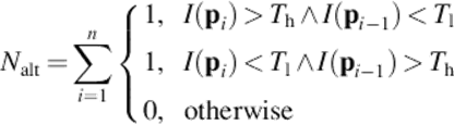
The first stage of the algorithm is the features detection. Corners x-shaped are identified analyzing the number of high-contrast alternations in the neighborhood of each pixel. Considering V = {p₁, p₂, …, p_n}, the neighborhood of a central pixel p_c defined by all pixels in the Breseham's circle border [19], the number of alternations is computed by Equation (1):

(1)

where p_i ∈ V, I(p_i) represents the pixel intensity of p_i, T_l and T_h are the inferior and superior threshold, respectively. Alternatively, both thresholds can be defined by: T_l = m − g and T_h = m + g, with .

The pixel p_c is classified as a x-corner if N_alt = 4 and T_l < I(p_c) < T_h. For Equation (1), when i = 0, i − 1 = n is assumed. Figure 1 shows the covered area by this detector.

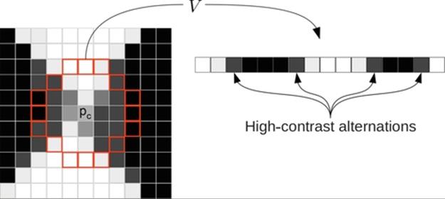
FIGURE 1 Typical neighborhood of a x-corner. Set V represents a circular border around central pixel p_c with four high-contrast alternations.

The variable g models the operator sensibility. Considering a previously blurred image, the number of alternations imposes large part of the restriction required for a proper classification. Thus the variable g has little effect on the final result. In this work, g is empirically defined with value 10.

This detector can be seen as a specification of the detector proposed in Rosten and Drummond [20], which is considered very fast. Since only a small portion of the neighborhood of the pixel is analyzed, the computational cost is reduced. Other similar detectors can be found in Zhao et al. [17] and Sun et al. [21]. Figure 2 shows a typical result of this detector over a chessboard image.

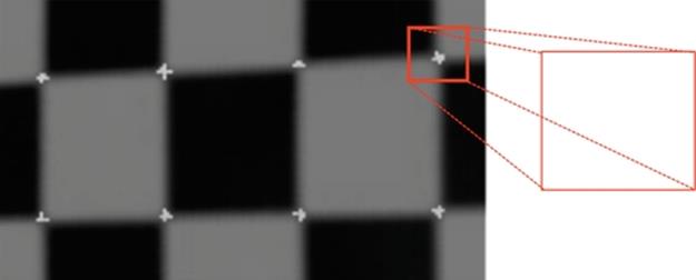
FIGURE 2 X-corner detector response. Light pixels define found corner positions in the image.

Equation (1) does not guarantee that only one pixel is classified as a x-corner in its neighborhood. To deal with this problem, the cost described by Equation (2) is associated with each corner and a nonmaximum suppression is performed [22].

(2)

The classes dark and light contains the dark and light pixels, respectively. The right corner is the one with the highest associated cost.

3 Topological filter

The identification of valid corners is an important step because not all x-corners present in the image belong to the calibration pattern. In this work, the identification of valid x-corners is made considering the regularity neighborhood of the chessboard image. This problem can be extended to the task of creating geometric meshes in computer graphics. In a mesh composed of basic components such as triangles, vertices are connected according to their neighborhood [23].

The Delaunay triangulation is a classic problem in computational geometry. Given a set of points in a plane, the only valid triangulation is one where the circumcircle of each triangle contains no other vertex [24]. This constraint ensures that the triangles are formed by the more closely vertexes. The mesh allows to define the neighborhood of each point. Figure 3 gives an example of this triangulation. Guibas et al. [25] present an algorithm for incremental triangulation that runs in time O(n log(n)).

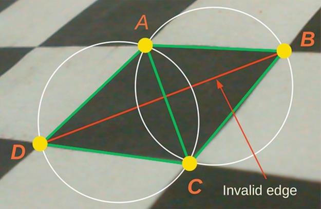
FIGURE 3 A Delaunay triangulation example. Considering A, B, C, and D four image corners, the valid triangulation if formed by the triangles Δ(A, B, C) and Δ(A, C, D).

Using the geometric mesh, the vertices and triangles are submitted to a topological filter to exclude those not satisfying the regularity of the pattern. The corners (or vertexes) share internal triangles of different colors in a regular manner. Each square of the chessboard pattern is represented by two triangles of the same color. Each triangle has no more than two neighboring triangles that form two squares with different colors alike. The internal vertexes have in common a maximum of eight triangles. Valid triangles have its interior filled with a single color.

Even after the projected image plane, the neighborhood relationship between the corners is still maintained. This restriction allows evaluating if corners really belong to the calibration pattern. Thus, are considered valid:

1. Those triangles that do not have color transitions in its interior;

2. Only those triangles that have a neighbor with the same color;

3. Those triangles that have only two neighbors of the same color and different color triangle taken as reference.

This filter is applied to the grid until there are no more invalid triangles. In the end, the vertices that do not form any triangle are also removed.

To avoid the use of thresholds in the comparison of colors, this filter uses a binarized version of the image. This is an important step to validate the points. If the binarization process fails, noisy points can be identified and actual points can be disregarded. To minimize these effects, this work uses adaptive binarization described in the work of Bradley and Roth [26]. This algorithm handles well with large variations in illumination and runs in linear time for any window size.

The binarization phase can be influenced by problems from the acquisition of images due to lighting variations and also by the fluctuation of the intensities of the pixels. In the regions near to the edges, a range of values may be wrongly considered black or white pixels. This behavior can generate white triangles with black borders and black triangles with white edges. In practice, the verification of color transition is made in a region of an innermost triangle, ignoring the edges. Figure 4 shows intermediate results of the algorithm including detected x-corners, initial mesh over the binarized image, and after the topological filtering.

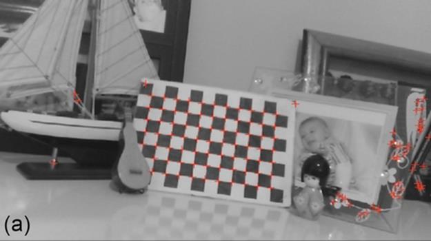
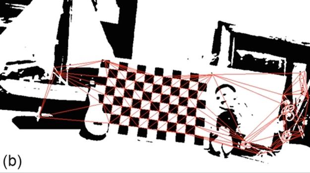
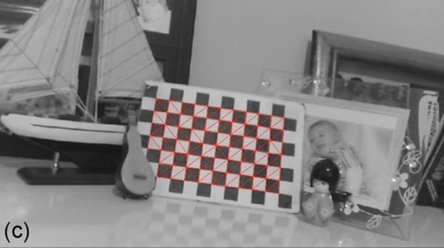
FIGURE 4 Mesh generation and topological filter results. (a) Initial x-corners, (b) triangulation over binarized image, and (c) valid triangles after topological filter.

4 Point Correspondences

The next step of the algorithm associates each vertex to the real coordinates of the pattern. This is done by analyzing the relative position of each corner. First two neighboring triangles of the same color are arbitrarily selected: T₁ and T₂. Three vertices make the triangle T₁, the origin of the coordinate system is defined by the vertex that has T₂ as its opposite triangle. For the remaining, vertices are assigned the directions x and y of the Cartesian plane (Figure 5).

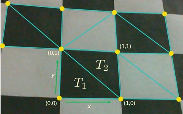
FIGURE 5 Propagation of coordinates. The triangles T₁ and T₂ define the origin and the direction of coordinates, respectively.

The propagation of coordinates consists in establishing the relative coordinates of the vertices neighbors. Given a triangle T whose vertices have already defined coordinates, where the origin is v_o, v_x and v_y are the vertices with the x and y directions, respectively. Triangle T_v is defined as a neighbor triangle of T with a different color. If triangles T_v and T are neighbors then they share an edge e and T_v has a opposite vertex to T, named v_v. The coordinates of the opposite vertex needs to be determined, thus:

1. If v_x ∈ e, then ;

2. If v_y ∈ e, then ;

It is understood by v^(⋅) the coordinate (⋅) of vertex v. Similarly, T_op shares a border e_op with T_v, then , where v_h is the third vertex of T_v and v_op is the opposite vertex to e_op.

For each visited triangle, the vertexes coordinates of the current and opposite triangles are propagated. The algorithm performs recursively for each neighbor triangle to the pair T_v and T_op. It makes the algorithm O(n/2), where n is the number of triangles in the mesh.

5 Location refinement

The x-corner detector, described in Section 2, identifies the position of corners with low accuracy where the only information available is the position of discrete pixels. Since the quality of the calibration is directly dependent to the precision which the position of features is found, there is a need for a refinement [1].

Traditional algorithms, such as Harris and Stephens detector [27] and Shi and Tomasi [28], run throughout the image and use thresholds to select the features of interest. The subpixel precision is achieved by maximizing functions fitted to the square of the intensity profile of the local neighborhood of each pixel. The threshold has a direct impact on the quality of response of these detectors, so corners are usually classified as the N pixels with greater response to the operator.

Chen and Zhang [4] propose a new detector specially designed to fit x-shaped corners. Considering the neighborhood of a pixel as a surface, its Hessian matrix can be expressed as:

(3)

where I_xx, I_xy, and I_yy are the second partial derivatives of pixel I(x, y). Thus, the x-corner detector is described as:

(4)

where λ₁ and λ₂ are the Eigen values of H.

In order to avoid unnecessary computation, this operator is only applied in regions defined by the valid vertices of triangle mesh. The real x-corner is the pixel with largest negative value of S and the refined coordinates [x₀ + s, y₀ + t]^T is given by:

(5)

6 Experimental Results

In this section, the detector response is evaluated considering an image database and by means of experimental tests with two different cameras. The image database is provided by the toolbox for MATLAB prepared by Bouguet [12]. This database consists of 20 images of a chessboard calibration pattern, accounting 156 x-corners arranged as 12 × 13 matrix, being presented in different orientations. This set represents a common situation to most of systems where the pattern images are first captured and calibration is performed in an off-line manner.

Figure 6 shows some examples of these images and Table 1 summarizes the results obtained for each one. The results are generated by applying the algorithm in each image and counting the number of corners identified. Analyzing Table 1, the vast majority of points is detected.

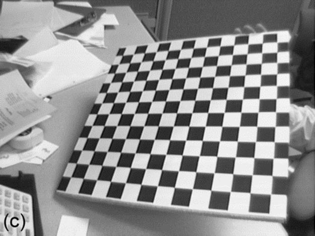
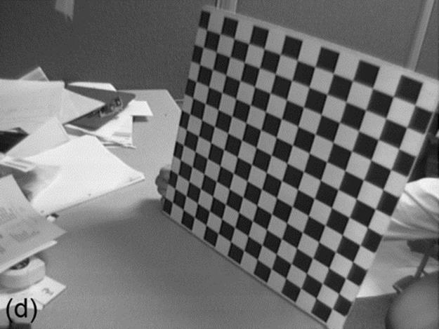
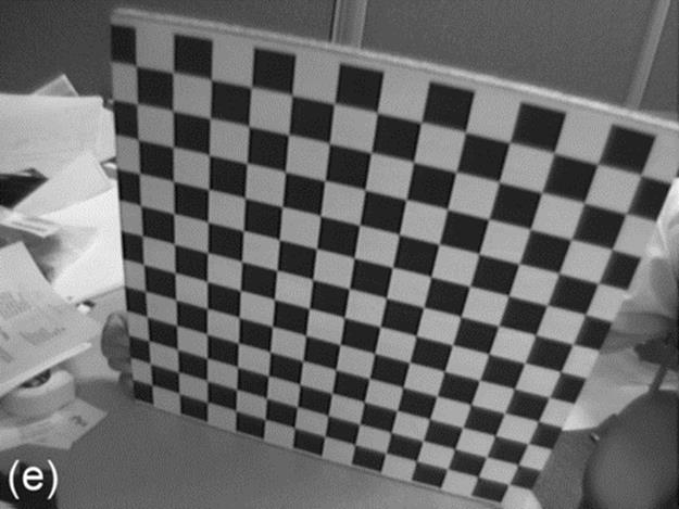
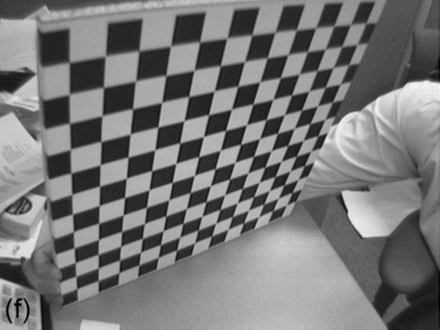
FIGURE 6 Examples of Bouguet database images. (a) Image 1, (b) image 2, (c) image 4, (d) image 9, (e) image 17, and (f) image 19.

Table 1

Results for the Bouguet Database

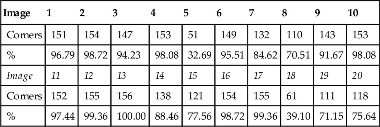
The rows named “Corners” list the number of detected x-corners and rows named “%” list the hit rate.

The mean accuracy of the algorithm is 85.38%; however, two images (images 5 and 18) require attention by the low percentage of detected points. They represent situations where the calibration plane is very inclined to the camera. In this case it is expected that the corners are uncharacterized by high perspective distortion and lack of focus in the image. Another aspect to be considered is that images in this database are of low contrast, which difficults the identification of alternations of high contrast. Figure 7 shows examples the best and worst for Bouguet images.

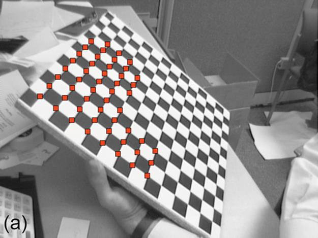
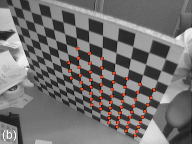
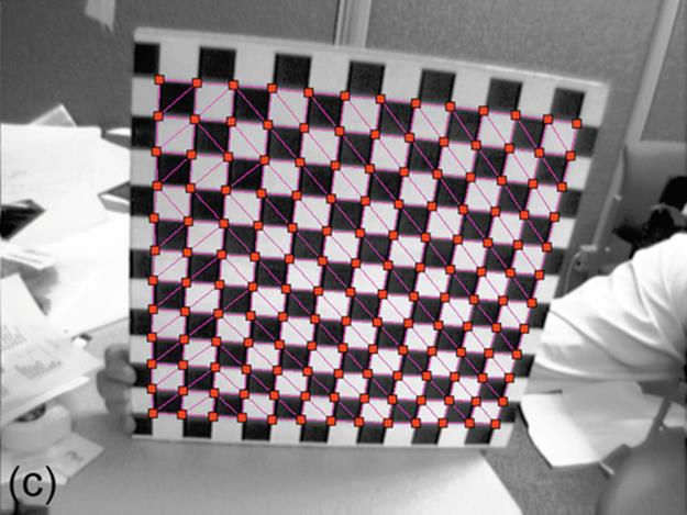
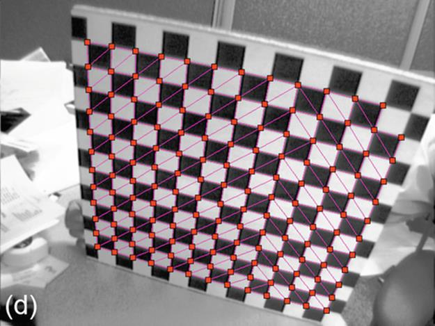
FIGURE 7 Worst (images 5 and 18) and best (images 13 and 17) result in the Bouguet database. (a,b) In images 5 and 18, few points are found due to pattern inclination. (c,d) In images 13 and 17, the pattern is fully detected.

In general, the algorithm was able to find the most calibration points. If the two worst images are discarded, the accuracy of success rises to 90.88%, which reflects the efficiency of the methodology. The absence of some points in the final result does not mean they were not detected. Both the presence of a false calibration point as the loss of a filter response influences on the neighborhood of these points. From a calibration perspective, where the presence of outliers affects substantially the camera parameters, it is more prudent to consider only those points that perfectly match with the regularity of the pattern.

For the online experiments, two different cameras were used: (1) Philips Webcam SPC990NC e and (2) Microsoft Webcam HD 5000. The calibration pattern used is formed by squares with 2.5 cm of width and forms a matrix of 11 × 7 x-corners. For each camera were tested 14 real images of the calibration pattern in various orientations and distances.

The algorithm runs on a sequence of captured frames. The amount of detected points presented in the second and fourth column of Table 2 corresponds to the average of the points detected in 10 frames for each position of the calibration pattern.

Table 2

Results for the Online Detection

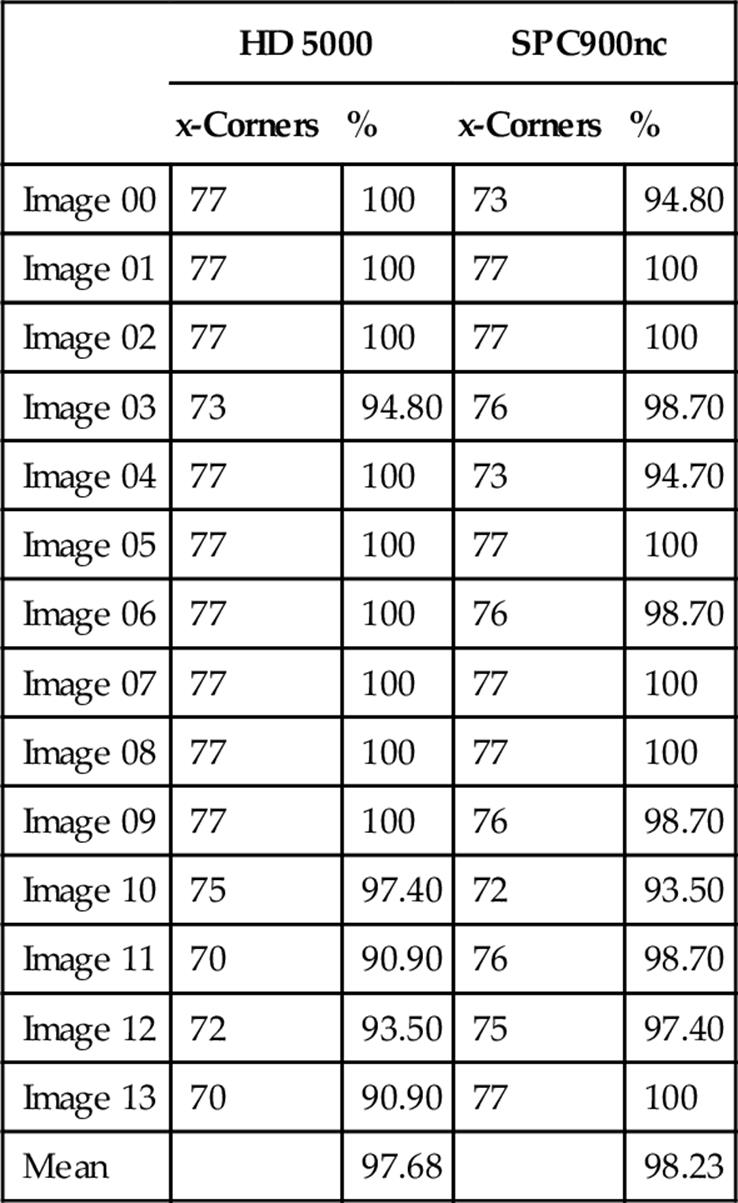
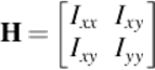
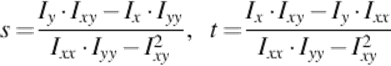
Figure 8 shows some of the images used in the second experiment. Once the pattern is completely visible, the algorithm has a high success rate, while the missed corners tend to arise when there is a more accentuated inclination of the plane in relation to the camera. In both experiments no false positives were identified, which confirms the robustness of the filter used. To illustrate the efficiency of the topological filter and propagation of coordinates, Figure 9 shows the result of the algorithm using complex backgrounds and partial occlusion of the pattern. The occluded corners do not interfere in the propagation of correct coordinates. Thus, it is possible to use the maximum of features identified for the estimation of camera parameters. The last column shows the reprojection plan calibration calculated from the detected points.

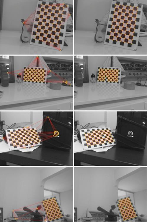
FIGURE 8 Example of images used in the second test. The left column shows all x-corners and the triangulation. The right column shows the topological filter result.

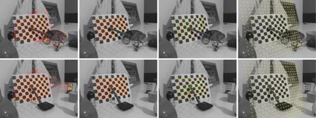
FIGURE 9 Results with complex backgrounds and partial occlusion.

7 Conclusions

This work proposes a methodology for automatic detection of chessboard calibration patterns. The algorithm runs automatically without any user intervention. It can detect the calibration points both in simple and complex background scenes where the calibration points mix with other image characteristics. The proposed methodology is robust to the presence of noise and also when the pattern cannot be fully identified. A partial identification of the pattern allows the calibration process to consider the max of detected points. In conditions where few points are available most picture frames are utilized.

References

[1] Hartley R, Zisserman A. Multiple view geometry in computer vision. 2nd ed. New York: Cambridge University Press; 2003.0521540518.

[2] Trucco E, Verri A. Introductory techniques for 3-D computer vision. Upper Saddle River, NJ: Prentice Hall PTR; 1998.0132611082.

[3] Dutta A, Kar A, Chatterji BN. A novel window-based corner detection algorithm for gray-scale images. In: Sixth Indian conference on computer vision, graphics & image processing, ICVGIP’08; Washington, DC: IEEE Computer Society; 2008:650–656. Available at:http://ieeexplore.ieee.org/lpdocs/epic03/wrapper.htm?arnumber=4756131 [accessed September 15, 2012].

[4] Chen D, Zhang G. A new sub-pixel detector for x-corners in camera calibration targets. In: 13th international conference in central Europe on computer graphics, visualization and computer vision, Winter School of Computer Graphics (WSCG-short papers)' 2005, Václav Skala - UNION Agency, University of West Bohemia. Plzen; Czech Republic: Citeseer; 2005:97–100. Available at: http://citeseerx.ist.psu.edu/viewdoc/download?doi=10.1.1.87.5833&rep=rep1&type=pdf [accessed November 8, 2011].

[5] Hu X, Du P, Zhou Y. Automatic corner detection of chess board for medical endoscopy camera calibration. In: Proceedings of the 10th international conference on virtual reality continuum and its applications in industry (VRCAI ’11); New York: ACM; 2011:431–434. Available at: http://doi.acm.org/10.1145/2087756.2087837.

[6] Krüger L, Wöhler C. Accurate chequerboard corner localisation for camera calibration. Pattern Recogn Lett. 2011. ;32(10):1428–1435. Available at: http://linkinghub.elsevier.com/retrieve/pii/S0167865511001024 [accessed November 28, 2012].

[7] Tsai RY. An efficient and accurate camera calibration technique for 3D machine vision. In: Proceedings of IEEE conference on computer vision and pattern recognition; 1986:364–374.

[8] Zhang Z. A flexible new technique for camera calibration. IEEE Trans Pattern Anal Mach Intell. 2000. ;22(11):1330–1334. Available at: http://ieeexplore.ieee.org/lpdocs/epic03/wrapper.htm?arnumber=888718 [accessed November 8, 2011].

[9] Hemayed EE. A survey of camera self-calibration. In: Proceedings of the IEEE conference on advanced video and signal based surveillance; 2003:351–357. Available at: http://ieeexplore.ieee.org/lpdocs/epic03/wrapper.htm?arnumber=1217942.

[10] Salvi J, Armangué X, Batlle J. A comparative review of camera calibrating methods with accuracy evaluation. Pattern Recogn. 2002. ;35:1617–1635. Available at: http://www.sciencedirect.com/science/article/pii/S0031320301001261 [accessed December 7, 2012].

[11] Bennett S, Lasenby J. ChESS—quick and robust detection of chess-board features. In: CoRR; 2013:1–13. [abs/1301.5] Available at: http://www-com-serv.eng.cam.ac.uk/~sb476/publications/ChESS.pdf [accessed May 6, 2013].

[12] Bouguet J-Y. Camera calibration toolbox for matlab (2008). http://www.vision.caltech.edu/bouguetj/calib_doc/.

[13] G. Bradski. Open computer vision library (OpenCV). In: Dr. Dobb’s J Softw Tools, 2000. http://www.opencv.willowgarage.com/.

[14] Fiala M, Shu C. Self-identifying patterns for plane-based camera calibration. Mach Vision Appl. 2007. ;19(4):209–216. Available at: http://link.springer.com/10.1007/s00138-007-0093-z [accessed May 21, 2013].

[15] De la Escalera A, Armingol JM. Automatic chessboard detection for intrinsic and extrinsic camera parameter calibration. Sensors. 2010. ;10(3):2027–2044. Available at: http://www.pubmedcentral.nih.gov/articlerender.fcgi?artid=3264465&tool=pmcentrez&rendertype=abstract [accessed November 28, 2012].

[16] Shu C, Brunton A, Fiala M. A topological approach to finding grids in calibration patterns. Machine Vision Appl. 2009. ;21(6):949–957. Available at: http://link.springer.com/10.1007/s00138-009-0202-2 [accessed June 25, 2013].

[17] Zhao F, Wei C, Wang J, Tang J. An automated x-corner detection algorithm (axda). J Softw. 2011. ;6(5):791–797. Available at: https://academypublisher.com/~academz3/ojs/index.php/jsw/article/view/0605791797 [accessed June 27, 2013].

[18] Laureano GT, Paiva MSV, Soares A.d.S. Topological detection of chessboard patterns for camera calibration. In: IPCV’13—the 2013 international conference on image processing, computer vision, and pattern recognition; 2013.

[19] Bresenham J. A linear algorithm for incremental digital display of circular arcs. Commun ACM. 1977;20(2):100–106.

[20] Rosten E, Drummond T. Machine learning for high-speed corner detection. In: Proceedings of the 9th European conference on computer vision—volume part I, ECCV’06; Berlin, Heidelberg: Springer-Verlag; 2006:430–443. Available at:http://link.springer.com/chapter/10.1007/11744023_34 [accessed June 23, 2013].

[21] Sun W, Yang X, Xiao S, Hu W. Robust checkerboard recognition for efficient nonplanar geometry registration in projector-camera systems. In: Proceedings of the 5th ACM/IEEE international workshop on projector camera systems (PROCAMS ’08); 2008:2:1–2:7. Available at: http://dl.acm.org/citation.cfm?id=1394625 [accessed June 25, 2013].

[22] Nixon MS, Aguado AS. Feature extraction & image processing for computer vision. 3rd ed. Oxford: Academic Press; 2012.9780123965493doi:10.1016/B978-0-12-396549-3.00002-1 p. 37–82.

[23] Bern M, Eppstein D. Mesh generation and optimal triangulation. Comput Euclidean Geom. 1992;1(1):23–90.

[24] de Berg M, Cheong O, van Kreveld M, Overmars M. Computational geometry: algorithms and applications. 3rd ed. Santa Clara, CA: Springer-Verlag TELOS; 2008.978-3-540-77974-2.

[25] Guibas L, Knuth D, Sharir M. Randomized incremental construction of Delaunay and Voronoi diagrams. Algorithmica. 1992. ;7(1-6):381–413. Available at: http://link.springer.com/article/10.1007/BF01758770 [accessed September 15, 2012].

[26] Bradley D, Roth G. Adaptive thresholding using the integral image. J Graph GPU Game Tools. 2007. ;12(2):13–21. Available at: http://www.tandfonline.com/doi/abs/10.1080/2151237X.2007.10129236.

[27] Harris C, Stephens M. A combined corner and edge detector. In: Taylor CJ, ed. Proceedings of the alvey vision conference. Alvey Vision Club. September 1988:23.1–23.6. doi:10.5244/C.2.23. Available at: http://www.bmva.org/bmvc/1988/avc-88-023.html [accessed May 22, 2011].

[28] Shi J, Tomasi C. Good features to track. In: Computer vision and pattern recognition. Proceedings CVPR ‘94., 1994 IEEE computer society conference on; 1994:593–600. doi:10.1109/CVPR.1994.323794. Available at:http://ieeexplore.ieee.org/xpls/abs_all.jsp=arnumber=323794 [accessed May 23, 2013].