Emerging Trends in Image Processing, Computer Vision, and Pattern Recognition, 1st Edition (2015)

Part III. Registration, Matching, and Pattern Recognition

Chapter 36. Distances and kernels based on cumulative distribution functions

Hongjun Su; Hong Zhang Department of Computer Science and Information Technology, Armstrong State University, Savannah, GA, USA

Abstract

Similarity and dissimilarity measures such as kernels and distances are key components of classification and clustering algorithms. We propose a novel technique to construct distances and kernel functions between probability distributions based on cumulative distribution functions. The proposed distance measures incorporate global discriminating information and can be computed efficiently.

Keywords

Cumulative distribution function

Distance

Kernel

Similarity

1 Introduction

A kernel is a similarity measure that is the key component of support vector machine ([1]) and other machine learning techniques. More generally, a distance (a metric) is a function that represents the dissimilarity between objects.

In many pattern classification and clustering applications, it is useful to measure the similarity between probability distributions. Even if the data in an application is not in the form of a probability distribution, they can often be reformulated into a distribution through a simple normalization.

A large number of divergence and affinity measures on distributions have already been defined in traditional statistics. These measures are typically based on the probability density functions and are not effective in detecting global changes.

In this paper, we propose a family of distances and kernels that are defined on the cumulative distribution functions, instead of densities. This work is an extension of our previous paper in IPCV’14 ([2]).

This paper is organized as follows. Section 2 introduces traditional kernels and distances defined on probability distributions. In Section 3, a new family of distance and kernel functions based on cumulative distribution functions is proposed. Experimental results on Gaussian mixture distributions are presented in Section 4. In Section 5, we discuss the generalization of the method to higher dimensional spaces. Section 6 provides conclusions and proposals for improvements.

2 Distance and Similarity Measures Between Distributions

Given two probability distributions, there are well-known measures for the differences or similarities between the two distributions.

The Bhattacharyya affinity ([3]) is a measure of similarity between two distributions:

In [4], the probability product kernel is defined as a generalization of Bhattacharyya affinity:

The Bhattacharyya distance is a dissimilarity measure related to the Bhattacharyya affinity:

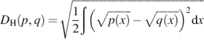
The Hellinger distance ([5]) is another metric on distributions:

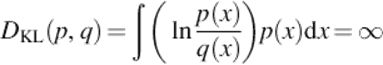
The Kullback-Leibler divergence ([6]) is defined as:

All these similarity/dissimilarity measures are based on the point-wise comparisons of the probability density functions. As a result, they are inherently local comparison measures of the density functions. They perform well on smooth, Gaussian-like distributions. However, on discrete and multimodal distributions, they may not reflect the similarities and can be sensitive to noises and small perturbations in data.

Example 1

Let p be the simple discrete distribution with a single point mass at the origin and q the perturbed version with the mass shifted by a (Figure 1).

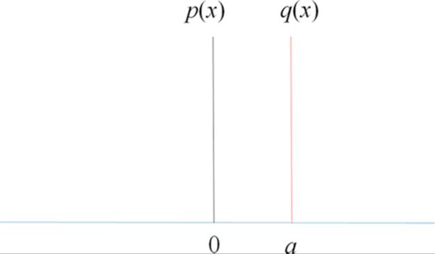
FIGURE 1 Two distributions.

The Bhattacharyya affinity and divergence values are easy to calculate:

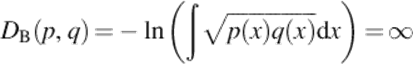
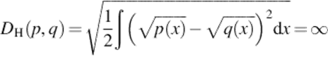
All these values are independent of a. They indicate minimal similarity and maximal dissimilarity.

The earth mover's distance (EMD), also known as the Wasserstein metric ([7]), is defined as

where Γ(μ, ν) denotes the set of all couplings of μ and ν. EMD does measure the global movements between the distributions. However, the computation of EMD involves solving optimization problems and is much more complex than the density-based divergence measures.

Related to the distance measures are the statistical tests to determine whether two samples are drawn from different distributions. Examples of such tests include the Kolmogorov-Smirnov statistic ([8]) and the kernel based tests ([9]).

3 Distances on cumulative distribution functions

A cumulative distribution function (CDF) of a random variable X is defined as

Let F and G be CDFs for the random variables with bounded ranges (i.e., their density functions have bounded supports). For p ≥ 1, we define the distance between the CDFs as

It is easy to verify that d_p(F, G) is a metric. It is symmetric and satisfies the triangle inequality. Because CDFs are left-continuous, d_p(F, G) = 0 implies that F = G.

When p = 2, a kernel can be derived from the distance d₂(F, G):

To show that k is indeed a kernel, consider a kernel matrix M = [k(F_i, F_j)], 1 ≤ i, j ≤ n. Let [a, b] be a finite interval that covers the support of all density functions p_i(x), 1 ≤ i ≤ n.

This metric is induced from the norm of the Hilbert space L²([a, b]). Consequently, the kernel matrix M is positive semidefinite, since it is the kernel matrix of the Gaussian kernel for L²([a, b]). Therefore, k is a kernel.

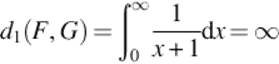
The formula for d_p(F, G) resembles the metric induced by the norm in L^p(R). However, a CDF F cannot be an element of L^p(R) because . The condition of bounded support will guarantee the convergence of the integral. In practical applications, this will not likely be a limitation. Theoretically, the integral could be divergent without this constraint. For example, let F be the step function at 0 and G(x) = x/(x + 1), x ≥ 0. Then

Given a data sample, (X₁, X₂, …, X_n), an empirical CDF can be constructed as:

which can be used to approximate the distance d_p(F, G).

When p = ∞, we have

The distance d_∞ is similar to the Kolmogorov-Smirnov statistic ([8]).

The distance measures defined above satisfy certain desirable properties of invariance.

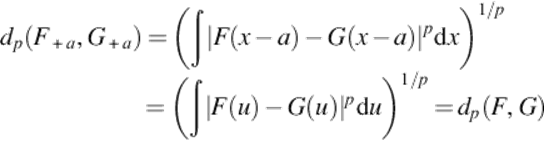
Proposition 1

d_p(F, G) is invariant under a translation. Let F_{+ a}(x) = F(x − a) be the CDF of X + a, a translation of the original random variable. Then

Proof

The CDF of X + a is F_{+ a}(x) = F(x − a)

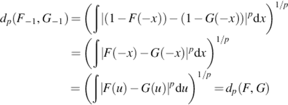
Proposition 2

d_p(F, G) is invariant under a reflection. Let F_{− 1}(x) be the CDF of − X, a reflection of the original random variable. Then

Proof

For a continuous random variable, F_{− 1}(x) = P(− X < x) = 1 − F(− x)

Proposition 3

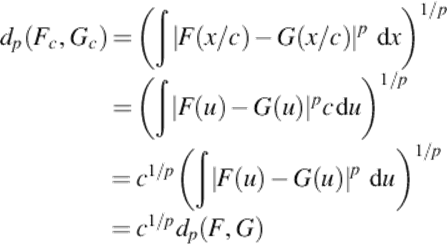
Let F_c(x) be the CDF of cX, c > 0, a scaling of the original random variable. Then

Proof

Example 2

Consider the same example as in the previous section. The CDFs of the distributions are illustrated in Figure 2.

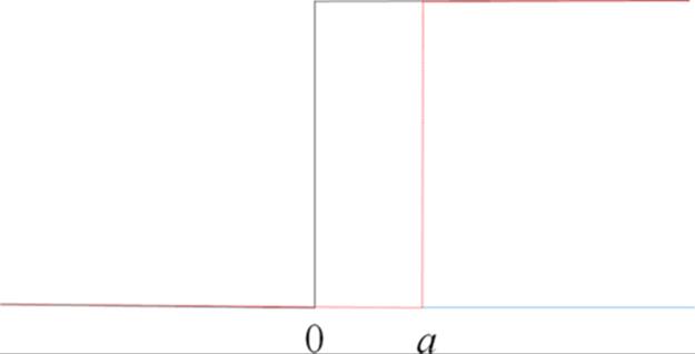
FIGURE 2 CDFs.

The proposed distance function has the value:

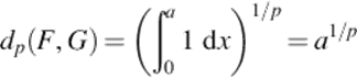
For p < ∞, the distance value is dependent on a. The kernel value is:

The computation of the distance d_p(F, G) is straightforward. For a discrete dataset of size n, the complexity for computing the distance is O(n). On the other hand, the computation of earth mover's distance requires the Hungarian algorithm ([10]) with a complexity of O(n³).

4 Experimental results and discussions

The CDF-based kernels and distances can be effective on continuous distributions as well.

A Gaussian mixture distribution ([11]) and its variations, shown in Figure 3, are used to test the kernel functions. The first chart shows the original Gaussian mixture. The other two distributions are obtained by moving the middle mode. Clearly the second distribution is much closer to the original distribution than the third one.

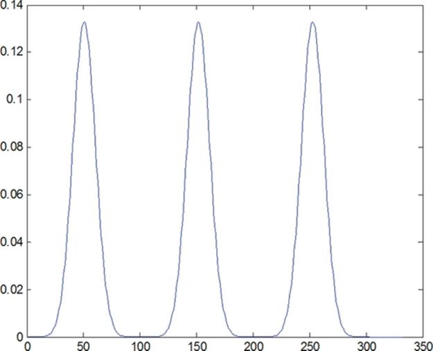
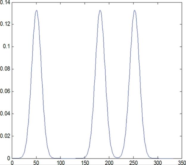
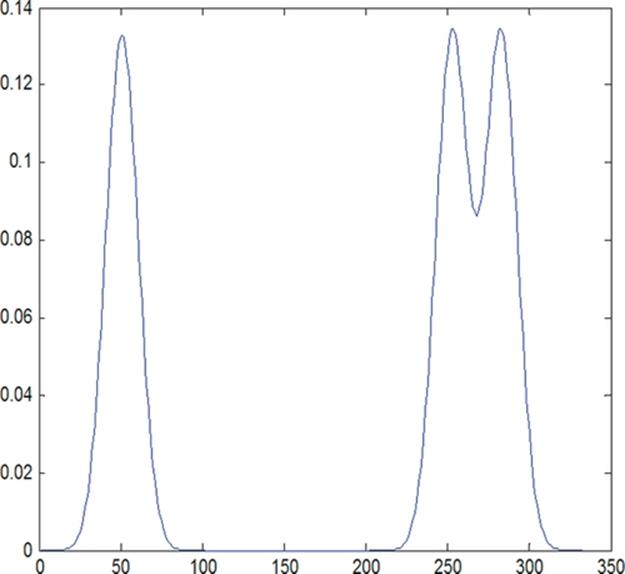
FIGURE 3 A Gaussian mixture and variations.

Indexed in the same order as in Figure 3, the Bhattacharyya kernel matrix for the three distributions is:

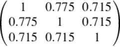
The Bhattacharyya kernel did not clearly distinguish the second and the third distributions when comparing to the original. There is no significant difference between the kernel values k₁₂ and k₁₃, which measure the similarities between the original distribution and the other two perturbed distributions.

The kernel matrix of our proposed kernel is:

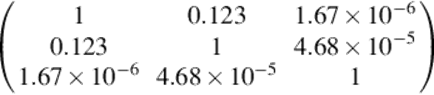
The CDF-based kernel showed much greater performance in this example. The kernel values k₁₂ and k₁₃ clearly reflect the larger deviation (less similarity) of the third distribution from the original.

This is due to the fact that the density-based Bhattacharyya kernel does not capture the global variations. The CDF-based kernel is much more effective in detecting global changes in the distributions.

5 Generalization

This method can be extended to high-dimensional distributions. Let F and G be n-dimensional CDFs for the random variables with bounded ranges. Then we can define the distance measures similar to the 1D case.

When p = 2, a kernel can also be defined from the distance d₂(F, G).

The advantages of CDF can be maintained in the high-dimensional cases. For example, the translation invariance and the scaling property can be established in a similar fashion. The 2D extension is especially interesting because it is directly associated with image processing. However, there exist challenges commonly associated with extensions to high-dimensional spaces. For example, there will be significant cost in directly computing high-dimensional CDFs. If m points are used to represent a 1D CDF, an n-dimensional CDF would need mⁿ points.

6 Conclusions and Future Work

In this paper, we presented a new family of distance and kernel functions on probability distributions based on the cumulative distribution functions. The distance function was shown to be a metric and the kernel function was shown be a positive definite kernel. Compared to the traditional density-based divergence functions, our proposed distance measures are more effective in detecting global discrepancy in distributions. Invariance properties of the distance functions related to translation, reflection, and scaling are derived. Experimental results on generated distributions were discussed.

Our distance measures can be extended to high-dimensional spaces. However, the calculation of distance using CDFs may incur heavy computational cost. For future work, we propose to develop an algorithm that computes the distance measure directly from the data, bypassing the explicit construction of CDFs.

References

[1] Boser BE, Guyon IM, Vapnik VN. A training algorithm for optimal margin classifiers. In: Proc. fifth annual workshop on computational learning theory - COLT '92; 1992:144.

[2] Su H, Zhang H. Distances and kernels based on cumulative distribution functions. In: Proc. 2014 international conference on image processing, computer vision, & pattern recognition; 2014:357–361.

[3] Bhattacharyya A. On a measure of divergence between two statistical populations defined by their probability distributions. Bull Calcutta Math Soc. 1943;35:99–109.

[4] Jebara T, Kondor R, Howard A. Probability product kernels. J Mach Learn Res. 2004;5:819–844.

[5] Hellinger E. Neue Begründung der Theorie quadratischer Formen von unendlichvielen Veränderlichen. J Reine Angew Math (in German). 1909;136:210–271.

[6] Kullback S, Leibler RA. On information and sufficiency. Ann Math Stat. 1951;22(1):79–86.

[7] Bogachev VI, Kolesnikov AV. The Monge-Kantorovich problem: achievements, connections, and perspectives. Russ Math Surv. 2012;67:785–890.

[8] Smirnov NV. Approximate distribution laws for random variables, constructed from empirical data. Uspekhi Mat Nauk. 1944;10:179–206 (In Russian).

[9] Gretton A, Borgwardt KM, Rasch MJ, Scholkopf B, Smola A. A kernel two-sample test. J Mach Learn Res. 2012;13:723–773.

[10] Munkres J. Algorithms for the assignment and transportation problems. J Soc Ind Appl Math. 1957;5(1):32–38.

[11] Bishop C. Pattern recognition and machine learning. New York: Springer; 2006.