Emerging Trends in Image Processing, Computer Vision, and Pattern Recognition, 1st Edition (2015)
Part III. Registration, Matching, and Pattern Recognition
Chapter 37. Practical issues for binary code pattern unwrapping in fringe projection method
M. Saadatseresht1; R. Talebi2; J. Johnson2; A. Abdel-Dayem2 1 Department of Geomatics Engineering, College of Engineering, University of Tehran, Tehran, Iran
2 Department of Mathematics and Computer Science, Laurentian University, Sudbury, Ontario, Canada
Abstract
A fringe projection system for three-dimensional (3D) reconstructions has been implemented and experimentation done with binary code pattern unwrapping based on time analyses approaches. The object under consideration is a sculpture of a woman. A step by step demonstration of the processes involved in fringe pattern projection on the object and 3D reconstruction of the object is presented. Evaluation was done by 3D printing the resulting point cloud and comparing the printed object with the original object. In the process of trial and error to obtain high-quality outputs at each step, an ideal setting was established for fringe pattern generation and fringe pattern photography. The requirements for achieving that ideal experimental environment are highlighted. Long-range objective is the implementation of 3D reconstruction on a handheld device (a less than ideal setting).
Keywords
Digital fringe projection
3D reconstruction
Phase unwrapping
Phase shifting
1 Introduction
Due to the growing need to produce three-dimensional (3D) data in various fields such as archeology modeling, reverse engineering, quality control, industrial components, computer vision and virtual reality, and many other applications, the lack of a stable, economic, accurate, and flexible 3D reconstruction system that is based on a factual academic investigation is recommended. As an answer to that demand, fringe projection has emerged as a promising 3D reconstruction direction that combines low computational cost with both high precision and high resolution. Research studies have shown [1] that the system based on digital fringe projection has acceptable performance, and moreover, it is insensitive to ambient light.
The major stages of fringe projection method are:
• A sinusoidal pattern is projected over the surface of the object by using a projector, as illustrated in Figure 1.
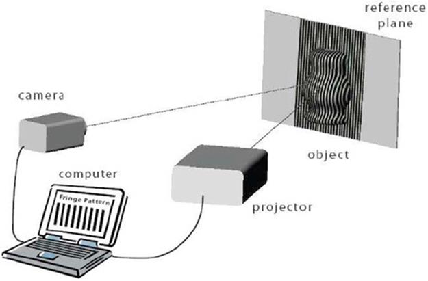
FIGURE 1 Fringe projection arrangement from [2].
• A digital camera is used to capture the pattern that has been phase modulated by the topography of the object surface.
• The captured pattern is analyzed to extract topographical information.
• A phase-unwrapping algorithm is executed to resolve discontinuities on the extracted phase.
• A phase to height conversion method is used to materialize the third dimension in every pixel.
Practical considerations regarding the fringe projection system in general and the binary code unwrapping method in particular are the focus of this paper. Section 2 highlights the previous research into fringe analysis. In Section 3, practical issues for fringe pattern generation are described. Section 4 describes the details of binary code generation for phase ambiguity resolution and evaluation of this unwrapping method. In Section 5, practical issues for fringe pattern photography are described. Section 6 offers concluding remarks and suggestions for future work.
2 Prior and related work
There have been many advances regarding structured light systems for 3D shape measurement such as multiple level coding, binary coding, triangular coding, and trapezoidal coding. Fringe projection 3D shape measurement improves upon the usual structured light systems because high-resolution (as high as camera resolution and projector) results in a correspondingly high speed. Furthermore, phase of each pixel, which includes modulated depth information, is calculated through gray-level intensities. The captured phase can be transformed to height (depth) for each pixel after discontinuities in the phase have been resolved by phase unwrapping.
Phase detection approaches have been based on a variety of approaches such as Fourier transform [3–6,14], interpolated Fourier transform [7], continuous wavelet transform [8–10,15], 2D continuous wavelet transform, discrete consign transform, neural network [11], phase locked loop, spatial phase detection, and phase transition.
3 Practical issues for fringe pattern generation
Fringe pattern generation is the process of projecting a sinusoidal pattern over the surface of an object and capturing the pattern by taking a picture of it with a digital camera. The object used for illustration is a chalky white sculpture of a woman without any sudden change in depth in its topography as shown in Figure 2.
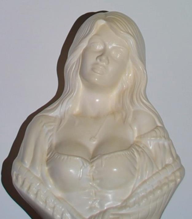
FIGURE 2 Object used for experimentation.
In our previous work [1], an experimental study and implementation of a simple fringe projection system have been reported that was based on a multiwavelength unwrapping approach. In that work, a classification of 3D reconstruction systems was also presented. In later work [12], a new method of phase unwrapping was implemented that is based on time analyses approaches. The fringe projection system provided an experimental environment in which the two unwrapping methods could be compared. Experimental results have shown that the digital code pattern unwrapping method is a stable and reliable method that results in a higher level of precision in the reconstructed 3D model at the cost of using more pictures. Using the same object to evaluate each unwrapping technique, it was found that binary code pattern unwrapping resulted in a more accurate point cloud.
Matlab high-level functions were used to produce the processing software to analyze the images and create the 3D models. Although there are other available choices of programming languages for image processing, Matlab has unique advantages for working in this field. In fact, we have created a magnificently powerful yet simple tool by taking advantage of Matlab's image processing capabilities. Processing functions will be described by showing fragments of Matlab code.
In the fringe pattern generation algorithm, creating the fringe patterns for one row will repeat for all the similar rows. Therefore, only one row of the algorithm will be explained. Assume that the projector has 100 width pixels. Assume that one fringe pattern is to be created with wavelength of 20 (T = 20), wave frequency of ω, three fringe shifts (N = 3), fringe shifting of 120°, and shifted phase value of p0. Accordingly, the phase P = ωt + p0 is a function of the pixel position (t = 1:n). The wave frequency is ω = 2π/T. Therefore, a0 + (b0-a0)*(1 + cos(P))/2 expresses a sinusoidal function with values between a0 and b0.
The brightness level of the fringe patterns in image pictures converts nonlinearly with the level of brightness in the projected patterns due to the radiometric behavior of the projector-camera system (Figure 3).
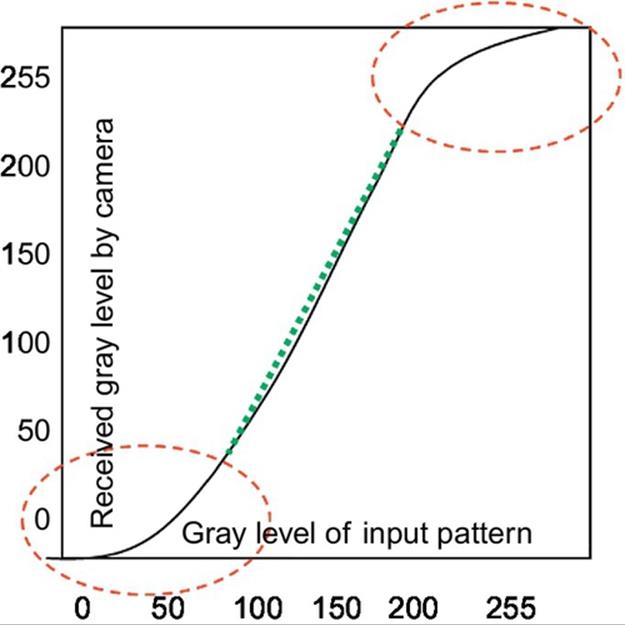
FIGURE 3 Photometric calibration of the projector-camera system. Red area: should not be considered in input gray level of pattern; dotted green line: middle area after gamma correction to make linear photometric projection function for the projector-camera system.
This nonlinear behavior will cause acute problems in producing the phase map. In order to avoid this problem, the range of black-and-white areas in the fringe patterns was changed from 0-255 to 50-200. Hence a0 and b0 were defined as a0 = 50 and b0 = 200. However, when working with shiny or very bright objects, defining the b0 value to 150 will help significantly reduce calculation errors and leads to better results in practice.
Phase P = ωt + p0 as a function of t is illustrated in Figure 4. The next step toward making the middle part of the function a linear photometric function is to do gamma correction. It is done by applying a calibrated exponential function on input gray levels or directly using a look-up-table between input-output gray levels. So we have:
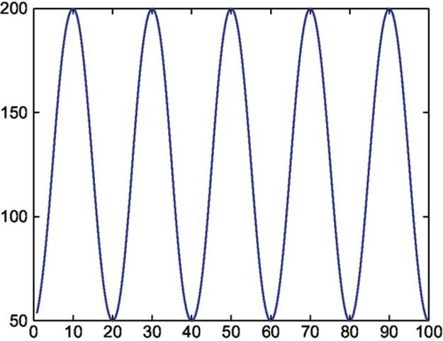
FIGURE 4 Calculated fringe patterns assuming values a0 = 50 and b0 = 150.
I = a0 + (b0-a0)*[(1 + cos(P))/2]∧γ which γ is the gamma parameter.
Considering the fact that by growing the t value the phase P will be increased, in immense values of P, Matlab will calculate the cos(P) with some volumes of errors, due to approximation of the Taylor expansion (truncation error).
Therefore, in calculating the phase P, it is better to calculate the value of function cos(P) after omitting the 2*k*π(2kπ) coefficients where k is an integer number used to count the number of coefficients of 2π. For calculating the reduced phase, the following code was used:
P = P-floor(P/(2*pi))*2*pi.
The fringe patterns should result in an 8-bit integer picture. Accordingly, the following command was used to convert the real I values to integer values:
I = uint8(round(I)).
Figures 4, 5, and 6 show the calculated fringe patterns function, shifted fridge patterns profiles (120°), and shifted fringe patterns for 0, 120, and − 120°.
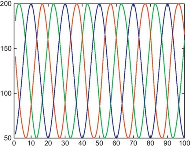
FIGURE 5 Shifted fringe patterns (120°) profiles in color.
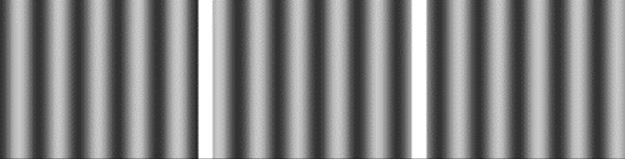
FIGURE 6 Shifted fringe patterns a: 0 b: 120 c: − 120.
As it is clear, changing p0 in relation P = ωt + p0 causes to shift the fringe pattern in x-axis. If it supposes γ = 0 then for each pixel, after projecting three patterns, there are three intensities:
I1 = a + b*cos (φ-2π/3)
I2 = a + b*cos (φ)
I3 = a + b*cos (φ + 2π/3)
Solving this equation set with three unknowns a, b, and φ (fi) gives us the output phase φ for each pixel individually:
fi = atan (sqrt(3)*(I1-I3)/(2*I2-I1-I3));
a = (I1 + I2 + I3)/3;
b = sqrt(3*(I1-I3)∧2 + (2*I2-I1-I3)∧2)/3;
a is the computed texture and b is data modulation. If b limits to infinity, then fi will be unstable and highly effected from noise so is not validate. It means the quality of the extracted fi depends on how far are the value of (I1-I3) and (2*I2-I1-I3) from zero.
After computation of wrapped phase φ, the final phase Φ = φ + 2kπ in which k is unknown ambiguity parameters. This ambiguity can be solved by different methods that will be described in the next subject.
4 Binary code generation for phase ambiguity resolution
Since phase modulation analysis uses the arctan function, it yields values in the range [− π,+π]. However, true phase values may extend over 2π range, resulting in discontinuities in the recovered phase and imprecision in the phase-unwrapping results. The procedure of determining discontinuities on the wrapped phase, resolving them, and achieving the unwrapped phase is called phase unwrapping.
Considering the fact that in each row, the fringe patterns will be repeated every 20 pixels, as a result, the phase ambiguity of each pixel will be increased with the amount 2*πi in each 20 pixels. In view of the above remark, if the phase ambiguity of each pixel is equal to k*2*π (2kπ), therefore k values will be distributed in k = 0-1-2-3-4. Generally, k goes from 0 to ceil (n/T − 1) giving k coefficients for phase ambiguity.
Assuming width of the projector equal to 1280 pixels (n = 1280) and 1280 pixels/20 pixels/area = 64 = 26 areas to be coded. Consequently, six binary pictures (code patterns) will be needed to code 64 areas.
The code value will be a number between 0 and 63 which actually is the 2π coefficients in phase ambiguity and can be used to unwrap the phase. It is mandatory to create one black and one white binary pattern in order to convert the gray-level pictures to binary. Hence, a threshold value should be defined based on the gray value norm and for each code if norm value is greater than the threshold, then it is going to change to one, otherwise it is going to change to zero. Therefore, the number of binary code patterns will be raised to eight as can be seen in Figure 7.
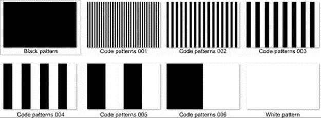
FIGURE 7 Binary fringe patterns: black pattern, code patterns 001-006, white pattern.
5 Practical issues for projected fringe pattern photography
Three crucial points should be considered regarding the optical arrangement and calibration in the projected fringe pattern photography:
• The position of the projector and camera should not be moved at all during the process of taking pictures. The camera should not be touched at all, and the pictures should be taken using a remote controller. These modest facts are significantly crucial in view of a very simple optical fact that if the camera lens moves one-hundredth of a millimeter, the picture pixels will move in scale of 10 or 20 (pixels) according to the distance between the camera and the reference plane.
• The projector and the camera should be focused on the object. Regarding the camera, it comes with better practical results if the camera setting be set on auto focus. Additionally, the projector should warp enough by choosing a precise focusing value that the pixels of the projected patterns on the objects should not be distinguishable from a near distance.
• The projector brightness level has to be chosen very precisely to avoid any distribution of the white lights fraction on the black part of the projected patterns on the object. The level of brightness can be set using the projector settings or by choosing smaller values (150 or even 100 instead of 255 as the gray values) for patterns on the brighter areas. These variables are mostly differing from one to other practical attempts. They are highly related to the level of brightness of the sculpture, how much light it will reflect, and how much dark or bright is the room or the wall behind the object.
Three fringe patterns and eight code patterns were created and projected on the object and reference plane separately. Figures 8 and 9 present the binary code patterns and projected fringe patterns on the object and reference plane, respectively.
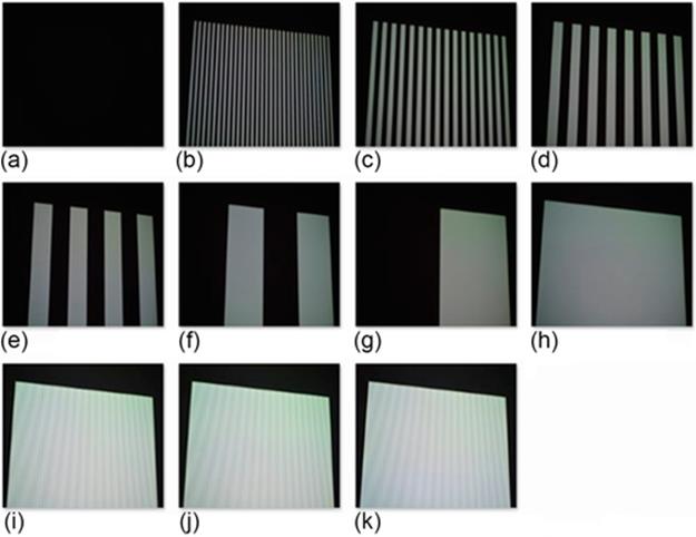
FIGURE 8 (a)-(h) Binary patterns projected on the reference plane. (i)-(k) Fringe patterns projected on reference plane.
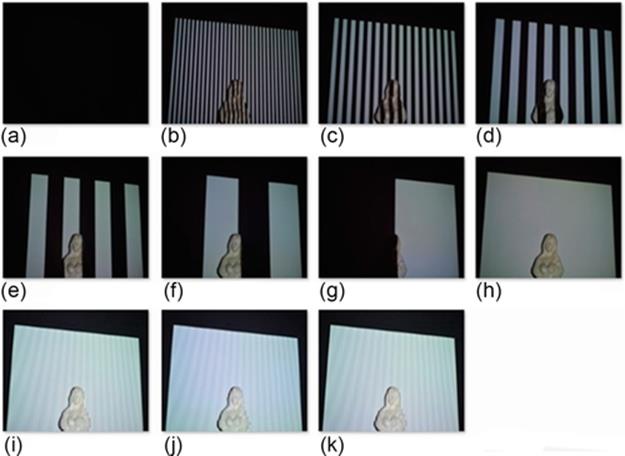
FIGURE 9 (a)-(h) Binary patterns projected on the object. (i)-(k) Fringe patterns projected on the object.
6 Three-dimensional reconstruction
It is possible to specify shadow areas using the fringe patterns. The threshold value for the mentioned operation is 20 using a 3 by 3 mask.
A=(I1+I2+I3)/3;
MSK=abs(I1-A)<TH & abs(I2-A)<TH & abs(I3-A)<TH
Figure 10 demonstrates the output resulting from applying the shadow recognition mask.
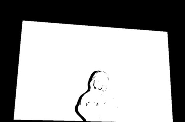
FIGURE 10 Shadow recognition output.
6.1 How to Compute the Initial (Wrapped) Phase
The wrapped phase can be calculated using the following command:
Wrapped Phase=atan2(sqrt(3)*(I1-I3),2*I2-I1-I3).*MSK;
Figures 10 and 11 illustrate ambiguity code of the scene before and after object placement (Figures 12–15).
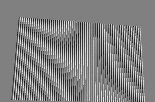
FIGURE 11 Reference plane wrapped phase.
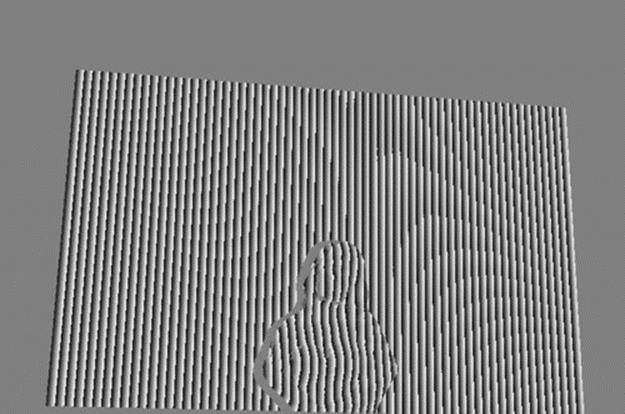
FIGURE 12 Object wrapped phase obtained by the phase-shifting fringe analyses method.
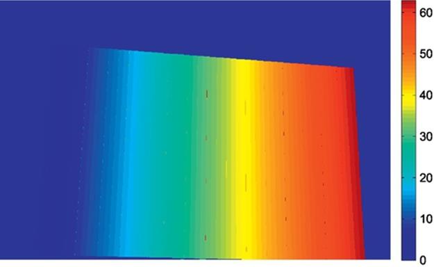
FIGURE 13 Retrieved reference plane code patterns.
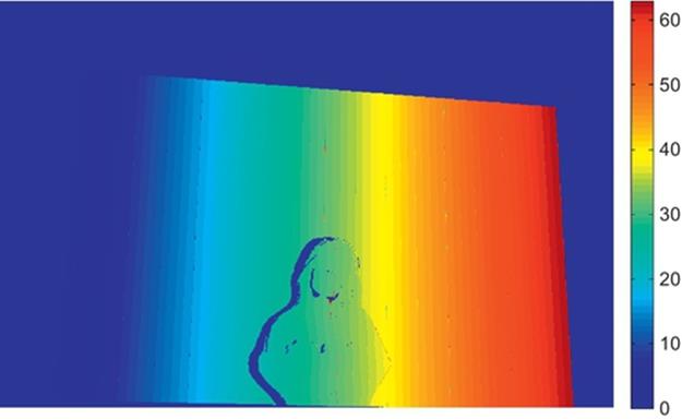
FIGURE 14 Retrieved object code patterns (0-63).
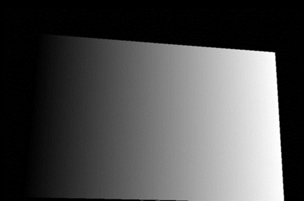
FIGURE 15 Reference plane unwrapped phase.
6.2 How to Compute the Unwrapped Phase via Two Previous Outcomes
Unwrapped phase=wrapped phase+code*2*pi
As can be seen in Figure 16, due to some minor errors in retrieving the code patterns in areas of varying white to black patterns, some artifacts have been created in the phase map.
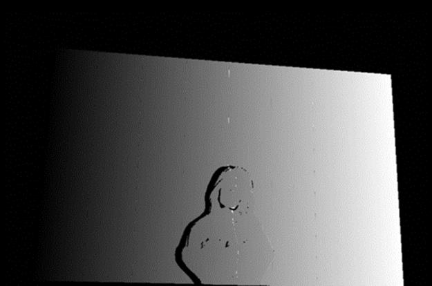
FIGURE 16 Unwrapped object phase with some artifacts.
6.3 Noise Removal from Unwrapped Phase
Because of problem in ambiguity code generation especially in boundaries of black-white areas, there are unwanted phase blunders (mistakes). We use median filter to detect these noises. If filter outcome has large difference with respect to the initial phase, we substitute it by the weighted average of neighbors. We can apply this filter several times.
ctdot;a=medfilt2(uwPhase,[1 7]);
c=filter2([1 2 3 0 3 2 1]/12,uwPhase);
b=abs(a-uwPhase)>(1.5*pi);
uwPhase = uwPhase.*~b+c.*b;
As can be seen (Figure 17), the median filter reduced the level of artifacts in significant scale. Compare Figure 16 before filtering with Figure 17 after filtering.
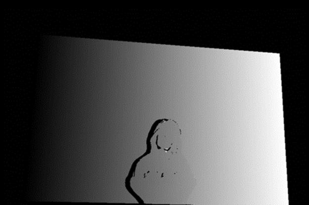
FIGURE 17 Unwrapped phase after median filtering to reduce artifacts.
6.4 Compute Differential Phase
Now object phase is subtracted from background phase using the following code to yield differential phase map of Figure 18. The depth can be computed after calibration of the differential phase image.
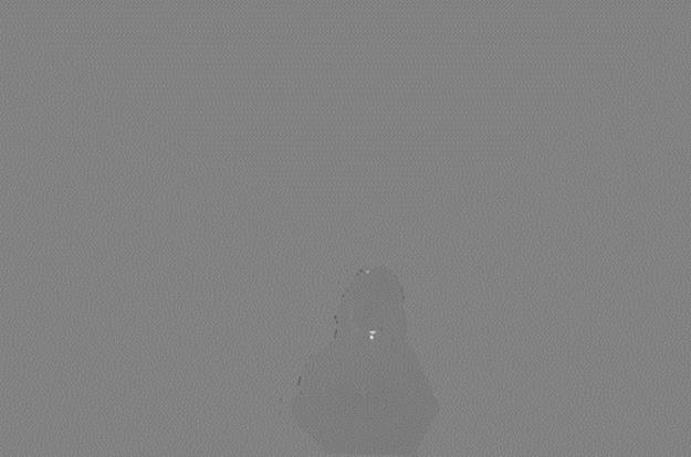
FIGURE 18 Phase map with some artifacts.
[p1,msk1,rgb1]=phaseproc(dir1,TH,FILTER);
[p2,msk2]=phaseproc(dir2,TH,FILTER);
dp=p1-p2;
msk=msk1.*msk2;
dp=dp.*msk;
6.5 Noise Removal from Differential Phase
As can be seen, the phase map (Figure 18) has very low contrast and object topography is not clear. This is because of phase mistakes with very large or very small values. Hence, we improved the previous phase map using the following filter:
dp(abs(dp)>15 | dp>-4)=0;
dpf=abs(dp);
After erasing these mistakes, we can see the much improved object topography in the phase map of Figure 19.
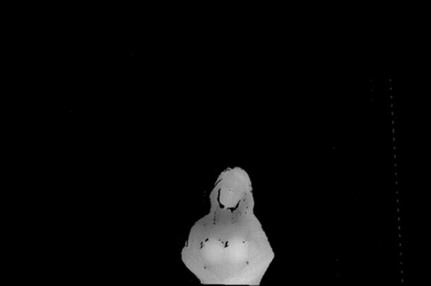
FIGURE 19 Phase map after filtering.
There are yet some phase errors especially at the edges. We can correct these errors using a filter previously used in phase computation. Like with phase computation, we can apply this filter several times by which we obtain the further improved phase map ofFigure 20.

FIGURE 20 Final phase map with modulated height information.
![]() a=medfilt2(dpf,[1 7]);
a=medfilt2(dpf,[1 7]);
![]() c=filter2([1 2 3 0 3 2 1]/12,dpf);
c=filter2([1 2 3 0 3 2 1]/12,dpf);
![]() b=abs(a-dpf)>.5;
b=abs(a-dpf)>.5;
![]() dpf=dpf.*~b+c.*b;
dpf=dpf.*~b+c.*b;
6.6 How to Make RGB Texture Image from Projected Fringe Pattern Images
RGB=(projected fringe pattern1+projected fringe pattern2+projected fringe pattern3)/3
As can be seen from the texture image of Figure 21, there are some unwanted periodic patterns and these could be removed by using phase filtering techniques in the frequency domain. However, a better method is possible as a result of binary code pattern unwrapping being used for ambiguity resolution. The idea is to use projected white code to obtain RGB texture image.
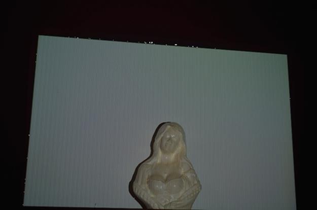
FIGURE 21 Object texture resulting from averaging operation.
6.7 Object Cropping
To diminish the size of point cloud data, we crop texture and phase images to object area (Figures 22 and 23) using the following code.
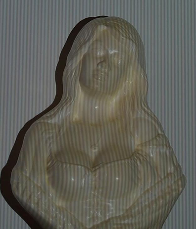
FIGURE 22 Cropped texture image.
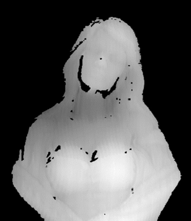
FIGURE 23 Cropped phase map.
xmin=1000;xmax=1600;ymin=900;ymax=1600;
dpf=dpf(ymin:ymax,xmin:xmax);
rgb1=rgb1(ymin:ymax,xmin:xmax,:);
To show colored depth map (Figure 24):
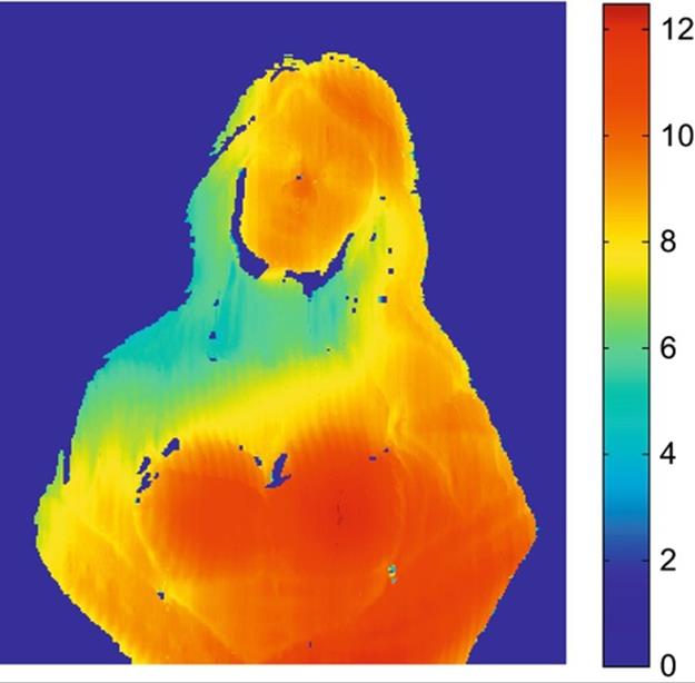
FIGURE 24 Colored depth map.
imshow(dpf,[])
colormap(jet(256));
colorbar
6.8 Convert Differential Phase to Depth and 3D Visualization
SC is scale factor to convert pixel value (phase) to depth (pixel unit).
[x,y]=meshgrid(xmin:xmax,ymax:-1:ymin);
x=x(dpf~= 0);
y=y(dpf~= 0);
z=dpf(dpf~= 0)*SC;
6.9 Accuracy Evaluation of 3D Point Cloud
Previously [1,12,13], the level of preciseness in the cloud point was revealed by direct observation of 3D visualizations. Here, cloud points are converted to inputs suitable for a 3D printer and precision is judged by comparison of the object printed with the original object that was to be reconstructed.
A variety of 3D mesh reconstructed models of the woman were created based on point clouds created by Matlab (e.g., Figure 25). Models were created by scientific/academic/trial version of “Geomagic” software. Many other programs are also capable of reading 3D (point cloud) file formats, for example, Microstation Point Cloud tools, Arc GIS Cloud Extension, and Mesh Lab to name a few. These applications are capable of providing the function to convert point clouds to many kinds of 3D models (e.g., wired mesh, 3D mesh) that can be used in applications with varying demands.
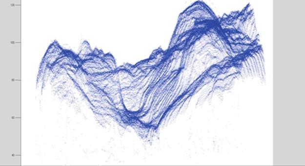
FIGURE 25 Woman sculpture point cloud created by Matlab.
Geomagic was used to create a 3D file in .stl format, a format that is supported by most of the mentioned point cloud analyzing applications and that can be read by a 3D printer. The workspace of the 3D printer (the cavity into which objects to be printed are placed) is limited and it could not house the original sculpture of the woman if we wanted to print it directly. A picture of the object printed from the .stl file is presented in Figure 26. The print size was arbitrarily specified to the 3D printer software to be one quarter the size of the original sculpture.
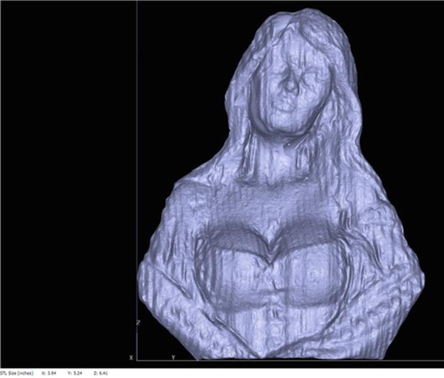
FIGURE 26 3D printing of point cloud of Figure 25 with STL size (inches) X = 3.94, Y = 5.24, Z = 6.41.
Left, right, and back views are given in Figures 27–29.
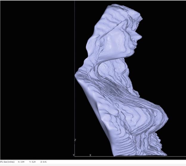
FIGURE 27 3D printing of point cloud left side view with STL size (inches) X = 3.94, Y = 5.24, Z = 6.41.
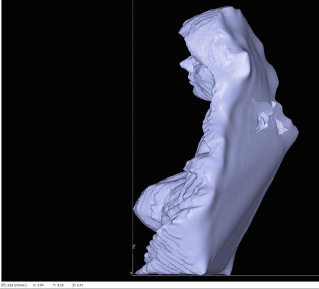
FIGURE 28 3D printing of point cloud right side view with STL size (inches) X = 3.94, Y = 5.24, Z = 6.41.
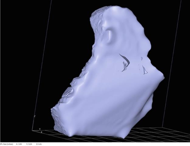
FIGURE 29 3D printing of point cloud back side view with STL size (inches) X = 3.94, Y = 5.24, Z = 6.41.
Imperfections are apparent in all of the 3D printings. There are holes in the neck area because there is so little information in that area being given to the printer. The thickness of the material used for printing, some kind of plastic inserted as cartridges in the 3D printer is greater than the depth information given by the point cloud in this region. The nose height is greater than the original object yielding a shape that is more pointed and not as round. That could have been introduced by the software for point cloud to 3D model conversion because this does not show up in previous renderings of the object.
7 Summary and conclusions
A new phase-unwrapping method, called binary code pattern unwrapping, was introduced and illustrated within a reconstruction system based on digital fringe projection. Along the way, practical issues had to be overcome and these and their solutions were enumerated. The fringe projection method, of which phase unwrapping is one step, was illustrated by showing the results obtained at the end of each stage of the process. The unwrapping method impacts results of later steps and binary code pattern unwrapping was found to produce a more accurate point cloud of the object in both depth and width directions compared with the previously studied multiwavelength unwrapping, but with tradeoffs.
In binary code pattern unwrapping, at least three shifted fringe patterns should be projected on the object. The projected fringe patterns should also have 120° phase difference. According to our practical results, the camera and projector should be close to each other, and the camera and projector optic axes should be parallel to the reference plane axis. Considering the mentioned optical calibration and system setting, three pictures should be taken from the object while the fringe patterns are projected on it. Next, the phase of the assorted patterns should be calculated. This process will be repeated with and without the presence of the object. In fact, it has been shown that the depth properties of the object can actually be calculated using the subtraction results of the object phase and the reference plane phase.
The main contributions reported here to ongoing research are as follows:
• Implementation and creation of practical parameterized experimental tools based on theories in the fringe projection method
• The development of a new phase-shifting process that reduces the number of pictures in fringe projection method
• Illustration that, by reducing the size of the fringe patterns, the level of preciseness of both height and details of the 3D model will increase
• Investigation of the optical arrangement of the fringe projection method and illustration by example of how failure in optical arrangement may cause failure in the whole method.
• Investigation of the reasons that may cause those errors concluding that in order to achieve the maximum level of preciseness, a controlled environment and precise metric equipment are mandatory.
Further research is expected, particularly with regard to the first contribution listed above with a view to creating a cellular device mobile scanner and a real-time scanning 3D measurement system. The richness of the Fourier transform method and the wavelength transition method that provide for modeling 3D phenomena has not been fully tapped by our approach. The mentioned methods have their own advantages in reducing the number of pictures and this may be beneficial in creating a real-time 3D modeling system. We have provided a general tool that applies to the phase-shifting fringe analyses method. A challenging problem for the near future is to provide more accurate, more stable, and more economic methods to create 3D models of any desirable elements of human life.
References
[1] Talebi R, Abdel-Dayem A, Johnson J. 3-D reconstruction of objects using digital fringe projection: survey and experimental study. In: Proc. ICCESSE 2013: international conference on computer, electrical, and systems sciences, and engineering; 714–723.World academy of science, engineering and technology. 2013;78.
[2] Gorthi SS, Rastogi P. Fringe projection techniques: whither we are?. Opt Laser Eng. 2010;48(2):133–140.
[3] Su X, Chen W. Fourier transform profilometry: a review. Opt Laser Eng. 2001;35(5):263–284.
[4] Tavares PJ, Vaz MA. Orthogonal projection technique for resolution enhancement of the Fourier transform fringe analysis method. Opt Commun. 2006;266(2):465–468.
[5] Li S, Su X, Chen W, Xiang L. Eliminating the zero spectrum in Fourier transform profilometry using empirical mode decomposition. J Opt Soc Am. 2009;A 26(5):1195–1201.
[6] Dai M, Wang Y. Fringe extrapolation technique based on Fourier transform for interferogram analysis with the definition. Opt Lett. 2009;34(7):956–958.
[7] Vanlanduit S, Vanherzeele J, Guillaume P, Cauberghe B, Verboven P. Fourier fringe processing by use of an interpolated Fourier-transform technique. Appl Opt. 2004;43(27):5206–5213.
[8] Dursun A, Ozder S, Ecevit FN. Continuous wavelet transform analysis of projected fringe patterns. Meas Sci Technol. 2004;15(9):1768–1772.
[9] Zhong J, Weng J. Spatial carrier-fringe pattern analysis by means of wavelet transform: wavelet transform profilometry. Appl Opt. 2004;43(26):4993–4998.
[10] Gdeisat MA, Burton DR, Lalor MJ. Spatial carrier fringe pattern demodulation by use of a two-dimensional continuous wavelet transform. Appl Opt. 2006;45(34):8722–8732.
[11] Tangy Y, Chen W, Su X, Xiang L. Neural network applied to reconstruction of complex objects based on fringe projection. Opt Commun. 2007;278(2):274–278.
[12] Talebi R, Johnson J, Abdel-Dayem A. Binary code pattern unwrapping technique in fringe projection method. In: Arabnia HR, Deligiannidis L, Lu J, Tinetti FG, You J, eds. Proc. 17th international conference on image processing, computer vision, & pattern recognition (IPCV'13); 2013:499–505 vol. I/II.
[13] Talebi R, Johnson J, Abdel-Dayem A, Saadatseresht M. Multi wavelength vs binary code pattern unwrapping in fringe projection method. J Commun Comput. 2014;11:291–304.
[14] Berryman F, Pynsent P, Cubillo J. The effect of windowing in Fourier transform profilometry applied to noisy images. Opt Laser Eng. 2001;41(6):815–825.
[15] Gdeisat MA, Burton DR, Lalor MJ. Eliminating the zero spectrum in Fourier transform profilometry using a two-dimensional continuous wavelet transform. Opt Commun. 2006;266(2):482–489.
All materials on the site are licensed Creative Commons Attribution-Sharealike 3.0 Unported CC BY-SA 3.0 & GNU Free Documentation License (GFDL)
If you are the copyright holder of any material contained on our site and intend to remove it, please contact our site administrator for approval.
© 2016-2026 All site design rights belong to S.Y.A.