Mastering Gephi Network Visualization (2015)

Chapter 5. Working with Filters

Filters are an essential component in Gephi, yet can be challenging to use compared with some of the other Gephi features. That's why we're devoting an entire chapter to the use of filters, one that will spend a minimal amount of space on theory before providing many examples on how to take full advantage of the power of filtering.

So why is filtering so critical for successful network analysis and graph creation? The simple explanation is that filters help to reduce the complexity and scope of large datasets, making them easier to navigate through and understand. The better answer is that filters can help improve our ability to tell stories and communicate with our data, as they allow us to focus on the critical elements in the network. This chapter will familiarize you with Gephi filters and what they can do, and then use multiple examples that demonstrate how to apply the filters and what the results look like in our networks. We will build on this knowledge at the end of Chapter 6, Graph Statistics, and begin employing filters on the statistical measures.

In this chapter, we will examine the following few key elements that are related to filtering:

· Advantages of filtering

· Primary filtering functions in Gephi

· Using simple filters

· Working with complex filters

Let's begin with a quick discussion of the filtering theory.

The filtering theory

You might be wondering why we should filter our network graphs in the first place. After all, it is possible to view entire networks using Gephi, and even to further navigate the same graphs using interactive tools. That's all well and good, but if you have been exposed to one of the hundreds (thousands?) of examples of overly dense, hairball-like graphs with no clear meaning, I believe you will quickly come to appreciate Gephi's ability to reduce visual complexity through the use of filters.

One of the beauties of filters lies in their ability to reduce complexity while not affecting the underlying data structure. All we are doing when we filter is removing unnecessary clutter from various stages of our exploration, including the final output. Filtering permits us to reduce the amount of guesswork and speculation about patterns and relationships by removing peripheral elements, thus permitting us to focus on the pieces that matter the most to our story. Think of a complex novel with more than 200 characters; should each character receive equal billing? Of course not. Yet when we produce graphs where it is difficult to tell the important members from peripheral actors, we have done our viewers a disservice.

Some elements can certainly be differentiated through adjusting their size, color, placement, and so on, but filtering provides a clarity that is difficult to achieve through any other means. By removing nonessential items from our field of vision, we also reduce the complexity and confusion that might impair the cognitive ability of viewers to interpret the graph. End users cannot draw conclusions about the elements that are not in the graph.

Filtering is also powerful from an analysis standpoint, as it enables you, as the graph builder, to be more easily exposed to patterns in the network, making it simpler to determine which elements belong in a finished graph. Rather than attempting to tell a single story from your network dataset, filtering can well lead you to multiple smaller insights that can contribute to a more compelling (and visually coherent) narrative.

These are the reasons we should filter our graphs, especially when they have any degree of complexity beyond the simplest of networks. With that said, let's transition to how we can use Gephi to build both simple and complex filters. Our first step is to become familiar with a wide range of filtering options that can be used alone or in tandem with other functions. Once we have become familiar with these functions, we'll begin using them on a dataset that details the interactions between students within a specific primary school environment.

Primary filtering functions in Gephi

Gephi filters are categorized into several groups, shown as individual folders in the Filters tab. Within each of these folders are multiple filtering selections that can be used on their own as simple filters, or combined to create complex filters. Primary filter categories include:

· Attributes: This folder houses many options that enable filtering on nodes, edges, partitions, clusters, and various graph measures such as eccentricity and various centrality levels. In addition, the user-defined attributes (such as a new column) can be found and acted on from this folder.

· Edges: This filter is applied strictly to the connections within the network.

· Operator: This filter allows you to execute a few functions on the graph.

· Topology: This filter offers a range of options where you can use graph measures such as degree ranges to filter the network.

Here's a screenshot showing the primary and secondary filtering folders:

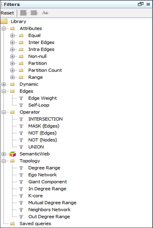
Filtering options in the Filters tab

Let's take a more detailed look at these folders so that we acquire enough understanding to spend time working with them on our example network. The next few sections separate the filters into groups just as they are laid out in Gephi. Not every filtering option is covered here. Additional options exist for semantic and dynamic filtering. While we won't explore them here, you should note that the dynamic filters can be used in instances where we have a time-based network where node and edge values are dynamic. The semantic filters can be used while working with RDF data structures such as SPARQL. For more information on RDF, you can visit the site http://www.w3.org/RDF/.

The following functions will nonetheless provide you with a powerful toolkit for navigating your network graphs.

Attributes

The Attributes filter allows you to query your graph based on the specific values within the network, including ID, Labels, Weight, and Modularity Class. This set of tools is highly useful when you wish to focus on a specific element of a group of values within the larger network. We'll provide basic instructions here for how you can expect these individual filters to operate, and then we'll work on them later in the chapter using some of the most essential ones on an actual dataset:

· The Equal function operates much as you might anticipate. Several options are available to take advantage of; for nodes, we can look for specific values based on Id, Label, or Modularity Class (assuming that you have clustered or partitioned your data). If we are looking to learn more about edges, then we can likewise use the ID and Label values, while also being able to specify the edge weight value to filter by.

· Inter Edges can be used to focus only on those edges that connect nodes within various partitions or clusters. This is particularly effective when the focus is on connections inside a group, and could certainly be used to shed light on networks with high levels of homophily. As is the case with other edge functions, one of the most compelling uses for this filter is to help clarify the connection patterns in an otherwise dense network.

· Intra Edges plays the opposite role to the Inter Edges functionality, highlighting only those connections that occur across groups. This will obviously be useful in cases where we are less interested in within the group communications, but are highly drawn to understand patterns between groups, and to determine which nodes are critical to these paths.

· The Non-null condition simply helps to hide missing values from the network graph, allowing us to focus on populated variables only. Options here are the same as for the Equal function we just discussed, giving us the ability to remove both nodes and edges that have missing values.

· The Partition filters are especially adept at creating custom views of individual partitions or clusters within the larger network, making it possible to quickly create subset versions of the entire network. Not only does this help in making the network more navigable for analysis, it also leads to visual results that can be far easier for viewers to comprehend.

· The Partition Count filter works on partitions as well, but does so using the counts within each partition, as opposed to the number that identifies each group. If our goal is to learn more on partitions with few members, the threshold can be set to remove larger groups from the graph, leaving us with only the smaller partitions being viewable. The opposite is true as well, if our focus is on heavily populated groups.

· With the Range filter condition, we have the capability to extend some of what was made available in the Equal filter. For instance, we can now specify a range of edge weights to display (say from 2 through 5). This can also be used to display a range of partitions in the same fashion, by differentiating this tool from the other partition filters.

Edges

A pair of edge filters exists beyond those already discussed in the Attributes section, which gives us the ability to further highlight desired patterns in the network that are mentioned as follows:

· If our goal is to examine or highlight a range of connection strength, then the Edge Weight filter is a highly useful tool. With this filter, all edge weights within specified minimum and maximum values can be highlighted, making it quite simple to draw attention to critical network paths.

· The Self-Loop filters can be applied in cases where a node connects with itself. This filter requires a subfilter (equal, partition, not equal, and so on) to activate the filter. We can then use these conditions to focus our attention on those nodes either with or without self-loops.

Operator

Several operator functions exist that can help us to build more complex filters. In our section titled Working with complex filters, described later in this chapter, we'll explore the practical use of these functions through a series of examples. In this section, our focus will be on providing a theoretical construct to help you understand when and how you might put each of these operators to use.

· The INTERSECTION operator enables the construction of highly complex filters using multiple conditions to narrow a network dataset. This can be thought of as resembling a database query where multiple conditions must be satisfied to return a set of records.

· MASK (Edges) can be used to customize the edges that are shown within a network graph. The filter provides four possible criteria via a set of radio buttons. These selections include any, both, source, and target.

· NOT (Edges) is used to remove certain edges from a view, either for practical or perhaps cosmetic reasons. As with the other operator functions, you must choose another filter for applying this criteria. For instance, we could elect to hide all of the edges that go across groups (inter edges), or conversely, all those within a group (intra edges).

· NOT (Nodes) can be employed to remove specific nodes from the network graph, and can be applied using other attributes that group the data, such as a class or other categorization. When used in this fashion, all nodes that belong to a specified group will be hidden from the view.

· The UNION operator is used to combine multiple conditions within a single data attribute. For example, in the case where we have categories from 1 through 25, we could use a union query to display both categories 1 through 5 and 20 through 25 while hiding the remainder. However with the other operator functions, we need to use separate filters such as Equal or Partition to build the union query.

Topology

Some of the most interesting filtering options are found in the Topology folder of the Filters tab. This is where you should go when you wish to learn more about the behaviors within the network, as opposed to focusing on highlighting specific elements within the network based on their specific group or position within the network. In this section, you'll learn more about how to navigate the network using a variety of filters that examine network structure and the role played by specific entities within the network.

· One of the starting points to understand influence within a network is to focus on the importance of specific individual nodes within the network. In Gephi, this can be done using the Degree Range filter, which enables filtering based on the number of connections each node possesses. In an undirected network, we are indifferent to the direction of the connection; in fact, it plays no role whatsoever. If the network is directed, then we can wish to defer to the In Degree Range and Out Degree Range options to better understand the patterns of influence within the network.

· Using the Ego Network function allows us to easily understand which other entities a single network node is connected to, at the first, second, third, and max degree levels. This allows us to see how the network is accessed by a specific individual working through the network and illustrates the possible paths required to access the second or third degree connections.

· The Giant Component filter enables users to hide portions of the network that are not part of the giant component or largest part of the network. In the case of a fully connected network, this filter will have no effect, but in other cases it will help to drive visual focus on the largest component in the network.

· We previously noted the In Degree Range filter, and how it can be useful to determine the levels of influence within a network. In a directed graph, this filter helps us to set thresholds that expose the nodes with the highest numbers of inbound edges from other nodes. This is a critical element for understanding which nodes serve as hubs and are relied on by other members for information or indirect connections.

· The Neighbors Network filter can be used in a similar fashion to the Ego Network filter, but with the ability to move beyond a single node. Thus, we can examine the neighbor network for a specific group within a network, rather than a single member, and extend it to include first, second, and third degree connections.

· The Out Degree Range filter lets us examine the degree to which nodes connect to other nodes; a sort of reverse hub effect if you will. While nodes with high levels of out degrees (relative to In Degrees) are typically not the influencers in a network, they might serve valuable functions as transmitters of information, acting as a conduit to many external information sources. The ability to isolate these nodes can help to understand the network structure and how information flows between members.

Using simple filters

For our purposes, we will define simple filters as consisting of a single filter placed on an element or attribute for the purpose of reducing the visual complexity of a network graph. The filter could be used to limit or highlight nodes, edges, partitions, or clusters in an effort to better understand and view structures within the larger network. To that end, we will devote this section to illustrate multiple examples for using simple filters to produce meaningful results that can be easily understood by the end users.

Even the so-called simple filters can help us uncover many intricacies in a network graph, particularly in cases where the network is too large to be easily deciphered by the naked eye. The following pages of examples are intended to walk you through the filtering process and provide an idea for what's possible even if you venture no further. Once again, we'll be using the primary school network to illustrate the power of simple filtering. This network can be found and downloaded fromhttp://www.sociopatterns.org/datasets/primary-school-cumulative-networks/.

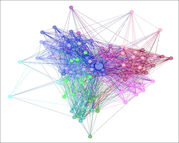
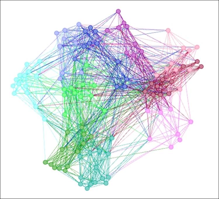
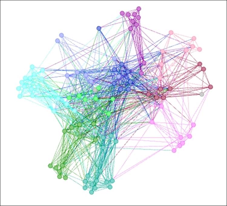
Let's start by looking at the entire network, colored by classnames:

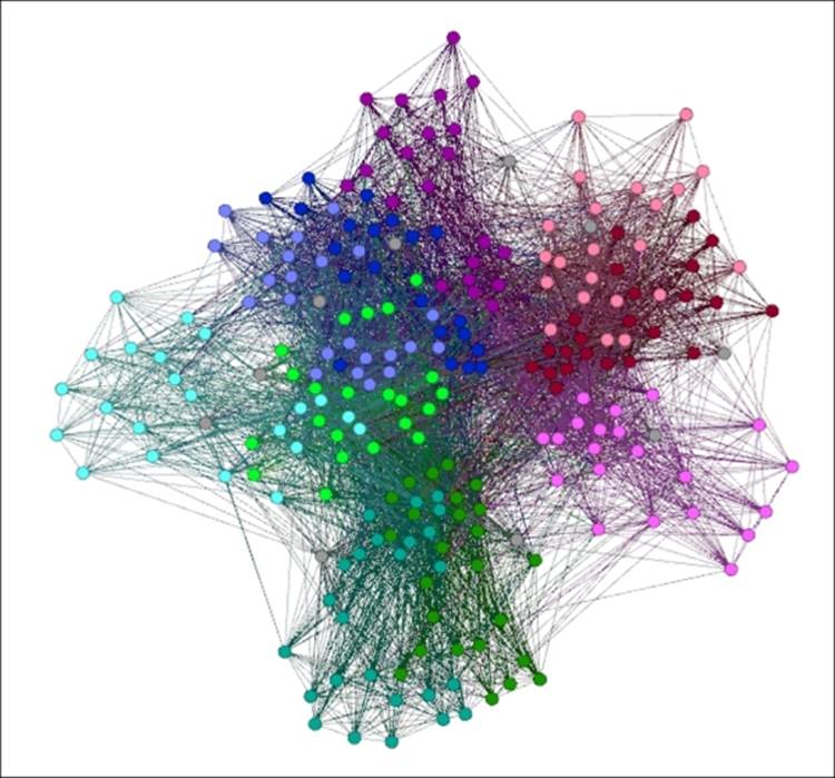
Entire primary school network

Even though this is not a large network, being composed of just 236 nodes, it still presents a visual challenge, in part due to the high degree of connectedness within the graph. We could simply choose not to show the edges, but we would then lose much of what makes the network unique. So our goal in the next few sections is to illustrate the value of filtering, not just for visual clarity, but also because we might well wind up seeing unanticipated patterns.

Using the Equal filter

We'll employ a host of filters to begin navigating the graph, starting with setting the gender attribute to female, by following these simple steps:

1. Navigate to the Filters | Attributes | Equal filter, and select the gender attribute.

2. Drag the gender attribute to the Queries space in the lower half of the Filters tab.

3. Set the value to F and run the Select and Filter options using the available buttons.

Your query settings should look like this:

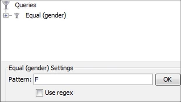
Filtering on gender using the Queries window

Here's our result after applying the filter:

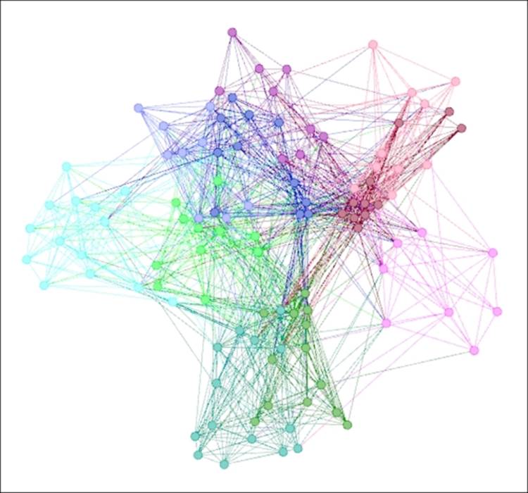
Primary school network filtered on female gender

While we haven't discovered anything too significant yet, the network has been thinned a bit which makes it somewhat easier to interpret. There are a couple of spots in the graph with very high density that might be worth investigating, but there is more we can do to query this network.

Let's remove the current filter (right-click on the filter and select Remove) and replace it with an instance where we become more selective with the data. Follow these steps to replicate the process:

1. Navigate to the Filters | Attributes | Equal filter and select the classname attribute.

2. Drag the classname attribute to the Queries space in the lower half of the Filters tab.

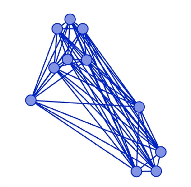
3. Set the value to 3B and run the Select and Filter options using the available buttons.

Here's our result:

Filtering on classname equals 3B

Now, we have something we can really focus on, as we have completely removed all the remaining classnames from the display. Notice the high degree of connectedness within this group, as well as the single node at the bottom-left, positioned some distance from the other classmates. This might provide a clue that this individual is more likely to be adjacent to some other classes, or perhaps acts as a bridge between classes.

Applying the regex function

Let's move on to another example using the same approach with a single difference. Certain Gephi filters enable the use of the Regular Expressions (Regex) function, which permits wildcards as part of the filter criteria. You probably already noticed this in the prior examples, and now we will take advantage of its capabilities. If you wish to learn more about using regex, visit http://www.regular-expressions.info/.

The only change we need to make is to replace the 3B value with 3 (3 followed by a period (.) symbol), followed by checking the Use regex checkbox. Now our filter will seek any instance where the classname starts with 3, which should return both 3A and 3B (think of this as similar to a LIKE statement in a database query). This will enable us to view the entire third grade to understand how much interaction occurs both within and across the two classes. Here's our graph:

Filter with classname equal to 3. using regex

Filtering edges

Let's switch from the Equal filter to the Inter Edges option, which will give us the opportunity to examine how nodes in one class link to those in another. To do this, we're going to remove the existing filter, and then apply the new one using the following steps:

1. Navigate to the Filters | Attributes | Inter Edges filter and select the classname attribute.

2. Drag the classname attribute to the Queries space in the lower half of the Filters tab.

3. Set the values to 1B and 2B by clicking on their respective boxes and then run the Select and Filter options.

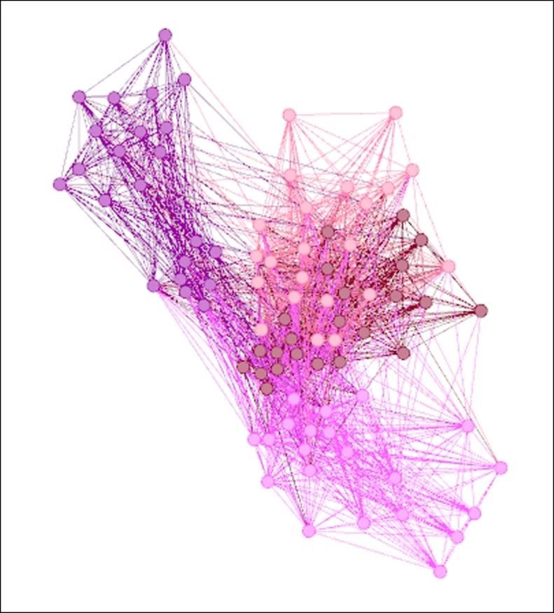
This will give us a look at the level of interaction between classrooms 1B and 2B—a single grade apart but presumably located in close proximity to one another:

Inter Edges filter on classnames 1B and 2B

It is quite easy to see that a considerable degree of interactivity occurs across these two classrooms. Notice also that this image is merely a subset of the entire graph, and the only portion with edges on display. There are some approaches that will also remove the remaining nodes from view, which will be covered in the next section on complex filters. For now, we can zoom in for better focus on our selected classes.

We have just seen the level of connectedness across these two classes, but what about within each class? To answer this question, we will simply replace the Inter Edges filter condition with Intra Edges, using the following steps (remember to remove the existing filter first):

1. Navigate to the Filters | Attributes | Intra Edges filter and select the classname attribute.

2. Drag the classname attribute to the Queries space in the lower half of the Filters tab.

3. Set the values to 1B and 2B by clicking on their respective boxes and then run the Select and Filter options.

Let's see what happens when this filter is applied:

Intra Edges filter on classnames 1B and 2B

Now we get an idea for how dense each class is—at first glance, it appears that connections within each class are much stronger than those across the classes. This can be verified using various graph statistics, which we'll introduce in Chapter 6, Graph Statistics.

Using the Partition filter

The Partition filter is another valuable tool that makes it very easy to select multiple values within an attribute. We'll demonstrate this in the following example. We'll begin by removing the existing filter, and then follow these steps to apply the partition conditions:

1. Navigate to the Filters | Attributes | Partition filter and select the classname attribute.

2. Drag the classname attribute to the Queries space in the lower half of the Filters tab.

3. Set the values to 4A, 4B, 5A, and 5B by clicking on their respective boxes and then run the Select and Filter options.

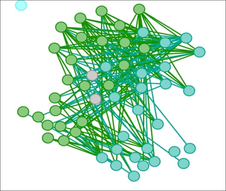
This will offer a view of the higher grade levels in the school and provide a first look at their patterns with respect to one another. Let's have a look at the resultant graph:

Partition filter on classnames 4A, 4B, 5A, and 5B

Here we get more interesting results, where there is some obvious overlap in the center of the graph composed of multiple classname members. Also of interest are the members at the lower-right and upper-left of the network, who appear to be less likely to interact with students from classes beyond their own.

Working with the Topology filters

To this point, our focus has been driven primarily by class levels. Now it's time to shift our focus to individual student behavior free from the somewhat artificial constraints of grade and class structures. This might also be a better way to understand critical behaviors within the network that are potentially being masked by group affiliations.

With that in mind, let's set our next filter using the following steps:

1. Navigate to the Filters | Topology | Degree Range filter.

2. Drag the filter to the Queries space in the lower half of the Filters tab.

3. Use the slider control to adjust the filter, moving the left slider to a value of 80 (or alternatively, type the value manually). Then run the Select and Filter options.

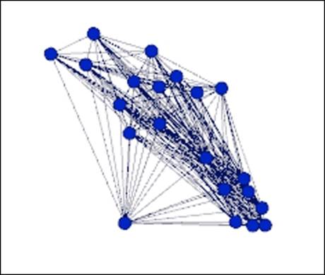
Our goal here is to reduce the viewable network to the most highly connected nodes so that we can observe who is most influential without having to cut through the visual clutter of seeing every member of the network. This will dramatically reduce the scope of the graph—your results should look like this:

Filter on degree range from 80 to 98

This simple filter reduced our graph from 236 to just 15 nodes. There are two immediate benefits to this approach. First, we can now easily identify the most highly-connected members of the network and simultaneously identify which classname they belong to, assuming that we have elected to partition the graph based on classname (you can read more on partitioning in Chapter 7, Segmenting and Partitioning a Graph).

Secondly, we can also detect connections between these influential members, which will shed a little insight into clustering patterns in the network. It does in fact appear that a majority of these nodes are connected with one another, which some of our statistical tests in Chapter 6, Graph Statistics, should pick up. In addition, we will learn how statistics can be recalculated after filters have been applied.

Let's go through two more quick examples before we move on to more complex filters. Our first example simply adjusts the filter settings from the previous example, as we seek to learn more about the least connected members of the graph. Use the slider to adjust the filter to return nodes with degree ranges between 18 and 30, and view the results:

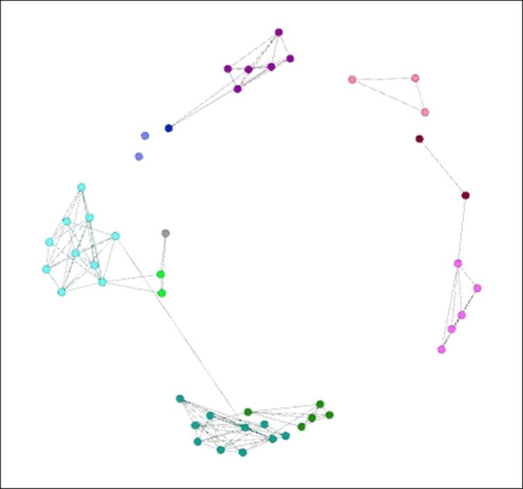
Filter on degree ranges between 18 and 30

As you might anticipate, the nodes with the lowest levels of interaction with the network are positioned around the perimeter of the graph. There are a couple of interesting patterns worth investigating from these results, with three of the classes having clusters that appear to be highly connected within the group, but are likely to have few external connections. While these don't appear to be perfect cliques where every node is interconnected, the patterns are still intriguing and can lead us to some interesting conclusions.

Our final example focuses on a single member of the network and his connections to others. Using the data laboratory, we have identified Node 1551 as the most highly connected member of the network, with a degree range equal to 98. This makes him a worthy candidate for further exploration as we attempt to understand his entire neighbor network and where they reside.

We're now going to explore the ego network for Node 1551. An ego network is simply the network of nodes that are connected to a single selected node. At a depth of one, we will see only the direct connections of the selected node, while a depth of two will show us all the second-level connections (the so-called friends of friends' network). To achieve this, we can employ the Ego Network filter, which can be applied using the following steps:

1. Navigate to the Filters | Topology | Ego Network filter.

2. Drag the filter to the Queries space in the lower half of the Filters tab.

3. Type the value 1551 in the Node ID box and leave the Depth setting equal to 1. Then run the Select and Filter options to see the first degree ego network for this node.

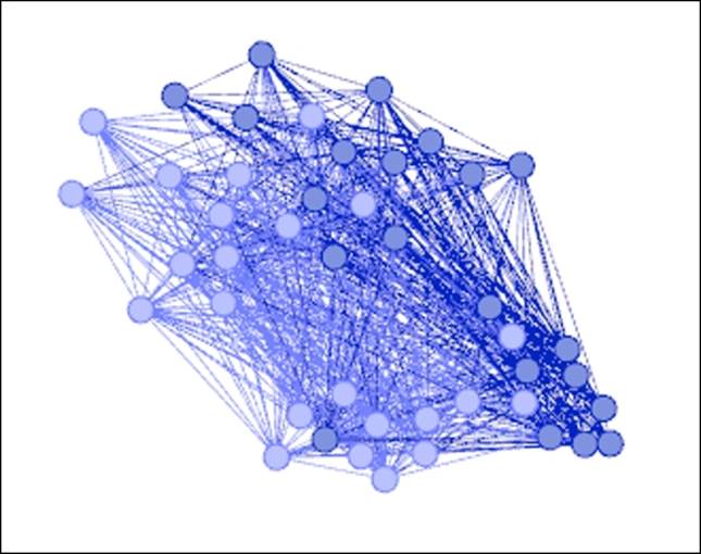
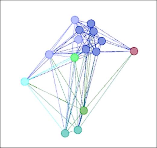
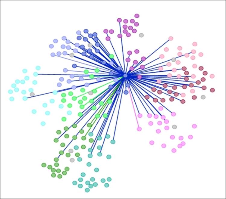
Here are the results, with Node 1551 manually resized for easier interpretation (you could also manually recolor for a similar effect):

Ego Network for Node 1551

Now we have an instructive view into the extent of Node 1551's influence across the network. While a majority of the connections are relatively close by, there are also some outliers at the perimeter of the graph, an indication that this particular student has interacted with a wide range of other students across multiple grades and classes. This might lead us to further investigate the reasons, if any, for this pattern. A similar analysis can be performed for any other node by entering the node ID in the filter.

By now, you should have a firm grasp of what can be done using simple filters. The benefits of filtering can be enormous, especially when we are encountered with dense networks that are difficult to decipher to the networks that are easily deciphered. Now the time has come to step up to complex filters where multiple conditions are combined in a single query.

Working with complex filters

Complex filters, for our purposes, are defined as filters with two or more conditions placed on some combination of nodes, edges, partitions, or clusters, once again for the purpose of focusing on a specific set of elements within a larger network. Using multiple filters in Gephi is not always easy or intuitive, so we will spend some extra time in this section to walk through several examples in order to expose both the complex filtering approach and the potential for further use of complex filters in your own graphs.

Applying multiple filter conditions

Let's start with some relatively simple examples, complex only in having more than a single filter. In this case, we will create one filter and then use a second condition as a subfilter to the first. Here are the steps:

1. Go to the Filters | Attributes | Equal filter and select the classname attribute.

2. Drag the filter to the Queries space in the lower half of the Filters tab.

3. Type the value 3B in the Pattern textbox and click on the OK button. You might also need to rerun the Select and Filter processes.

4. Now repeat step 1 using the gender attribute and drag it to the subfilter area of the initial filter.

5. Enter the value F in the textbox and click on OK. Our settings should look like this:

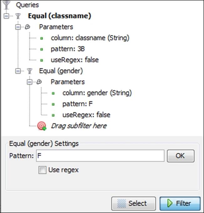
Using an equal filter with a subfilter

We should now see the following result in your graph window:

Nodes filtered by classname equals 3B and gender equals F

We now have a graph that has been quickly reduced to just 11 nodes of the original 236 by merging two simple filters. From here, we can easily change the classname value or the gender value that allow us to filter the network in a rapid fashion. This filter could also be saved for later use by right-clicking on and selecting Save, which will park the filter in the Saved queries folder. Let's move to another example; this time we will cover an example that combines three separate filters into a single query by using the subfilter capability.

Using subfilters

This time we'll really narrow our graph down by merging three filters as follows:

1. Go to the Filters | Attributes | Partition filter and select the gender attribute.

2. Drag the filter to the Queries space in the lower half of the Filters tab.

3. Select the F value by clicking on the adjacent rectangle and click on the Select and Filter buttons. You'll now see only female members of the network.

4. Go to the Topology | Degree Range filter and drag it to the subfilter section of the gender filter we just created. Now adjust the value to a minimum of 60 by using the left slider or by entering text.

5. Navigate to the Operator | NOT (Nodes) filter and drag that to the subfilter area of the degree range filter we just created.

6. Go back to the Partition filter and select classname.

7. Drag classname to the subfilter area of the NOT (Nodes) filter.

8. Run Select and Filter using the usual buttons.

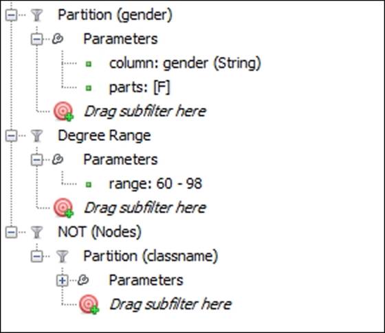
Here's what our filter should look like:

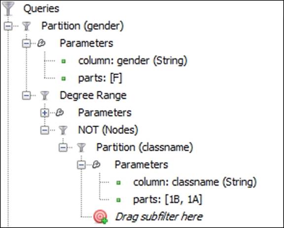
Complex filter that combines gender and degree range excluding the classnames 1A and 1B

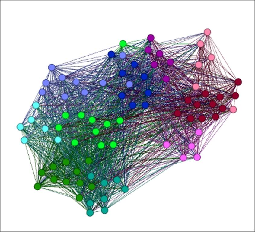
We now have a filter that identifies all highly connected female members of the network who are not in classnames 1A or 1B. Here's our result:

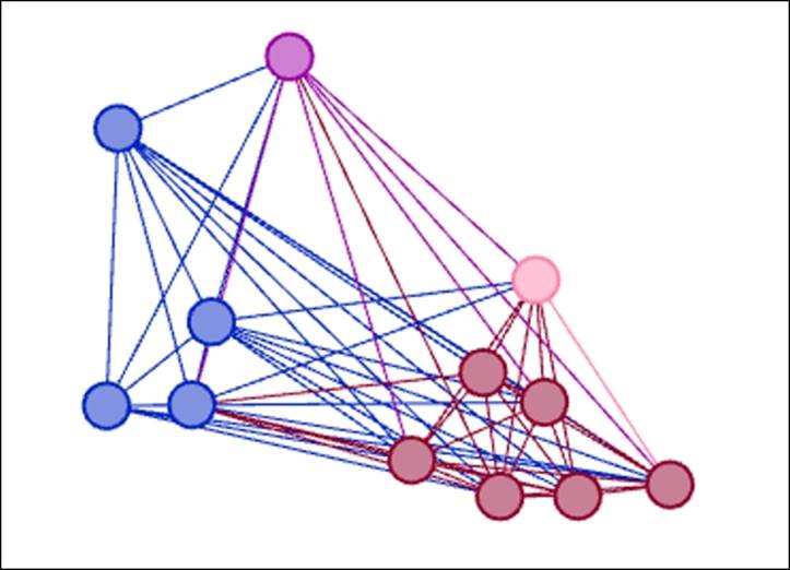
Results of filtering on female, degree range of 60-98, and not in 1A or 1B

You can see how quickly we whittled the network to just 12 nodes by combining these three conditions. From here it's also easy to tweak the settings—perhaps we would like to view only the 10 most connected female students. Simply increasing the degree range threshold will enable us to see these results refreshed with the new conditions. In fact, if we increase this value from 60 to 62, we are left with just nine students who meet all three criteria.

What would happen if we hadn't nested these criteria in a single query, but had chosen to isolate each filter? You can probably guess what the results will look like. Here are the three filter conditions we just presented, but now they act as standalone queries:

Individual filters not nested in a single query

To create this query, simply follow the same steps we previously used, with one exception. Rather than nesting each filter inside another as a subfilter, this time add each one as its own query, as shown in the preceding screenshot. Run them one at a time by clicking on the Select and Filter buttons.

First, we'll run the Partition filter with the value set to F, which results in the following graph:

Filtering on partition equal to F

As you might have anticipated, the network has been reduced to roughly half by hiding all nodes with gender equal to male.

Next, we'll filter on Degree Range, to identify all network members ranging between 60 and 98 degrees. Make sure the lower value is set to 60, and then filter the results to see the following output:

Filtering on degree range between 60 and 98

Now you are seeing only those nodes with a degree level of 60 or greater, including both male and female members. The prior filter is effectively overwritten by the new condition, rather than combining them as we previously saw. To verify that this is the case, go toData Laboratory and view the results to confirm the presence of both male and female students.

Let's apply our third filter—the NOT (Nodes) operator that excludes classnames 1A and 1B. You should see the following results:

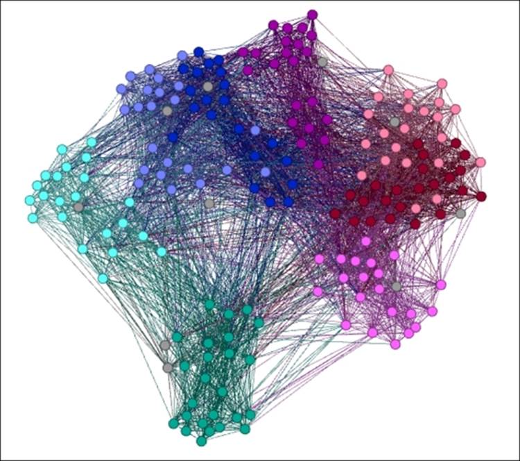
NOT (Nodes) with partition on classname equal to 1A and 1B

Not only do we have both genders visible in our dataset, but also students from the entire degree range from 18 through 98. The only missing members are those from classnames 1A and 1B, which can be confirmed by viewing the Data Laboratory results.

So while these individual filters can obviously not be used in the same manner as the nested versions, they do have a considerable value. If you wish to filter your network across many conditions then simply set those up in the Queries window, and then you have the ability to toggle through an array of filters to learn more about your network. Think of it in the same way as a statistician might work with single variable crosstabs to learn more about a dataset before moving on to a higher level of complexity.

Working with Mask and Intersection conditions

Now let's tackle our remaining examples, starting with an instance where we will focus on the ego network of an individual student. To complete this example, we'll work with the INTERSECTION filter, found in the Operator folder within the Filters tab, as follows:

1. Apply the Ego Network filter found in the Topology folder of the Filters tab. Follow the usual process of dragging the filter to the Queries tab, and then setting Node ID to 1551. Run the filter to get the initial results. This might appear a bit messy at this point, but we're going to take care of that in a moment.

2. Next, locate the MASK (Edges) filter found in the Operator folder of the Filters tab. Things get a bit trickier here, but we'll recap our steps at the end of this section. Drag the filter to the Queries tab as a standalone filter. Then add the Id filter from the Equalfolder. Make sure you select the node version, rather than the edge filter. Add this to the subfilter area of the MASK (Edges) filter and set the value to 1551, just as we did in our initial filter (we need these values to agree with one another). By the way, your graph will still look a bit untidy at this stage.

3. Next, repeat the process we just did with the Id (Node) filter by dragging it to the subfilter section of the first Id filter. Set the value to 1551 yet again. Now your graph should look quite different—a network with many nodes (98 to be specific) but with no connecting edges. To make the edges appear, we need to create an intersection between our filter conditions.

4. To complete the process, drag the INTERSECTION filter from the Operator folder down to the Queries tab. Make sure it is standalone at this point. Then drag the original filters one at a time into the subfilter area of the INTERSECTION operator. Set theMASK (Edges) setting to any by selecting the corresponding radio button, and run the Select and Filter processes. If you have taken a look at an intermediate stage, you might have seen something along these lines, with extra nodes that are not part of the ego network:

Ego Network with masked edges, intermediate stage

Your finished graph will resemble the following graph, with the remaining nodes filtered out of the process, and all first degree connections displayed like this:

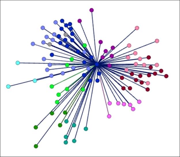
Completed ego network with masked edges

Here's a screenshot for how your complete query will appear:

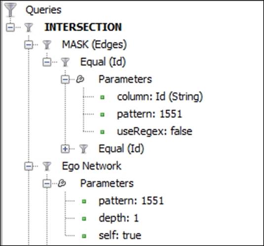
Intersection of masked edges and ego network

Remember to set the second (redundant) Equal (Id) value to make sure that the filter operates as expected. This might seem slightly quirky at first, but once learned, it becomes simple to apply to many other examples.

Working with the UNION operator

Now that we have run through a fairly complex example using the intersection logic, we'll end the chapter with an instance using the UNION operator. If you think of intersections as being parallel to the use of AND constructs in database queries, then unions are much closer to the OR condition. One notable difference is the requirement that union queries to get based on a single data attribute, where intersections derive their power from merging conditions across multiple attributes.

Given that this example is easier to follow than the last, we'll first introduce the filter conditions of the filter that we are creating, and then view the results. Here's how we want our filter to appear, which can be achieved by performing the following steps:

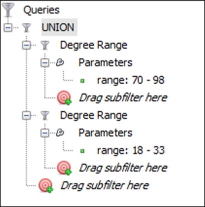
Union query with low and high degree ranges

To create the filter, follow these steps:

1. Go to the Filters | Topology | Degree Range filter and drag it to the Queries tab.

2. Repeat the same process by dragging the second filter to the Queries tab as a standalone instance.

3. Set the first Degree Range filter to a minimum value of 70.

4. Set the second filter to a maximum value of 33.

5. Go to the Filters | Operator | UNION filter and drag it to the Queries tab as a standalone item.

6. Drag each of the two filters to the subfilter area of the UNION operator, similar to what we did with the intersection example.

7. Run the filter using the Select and Filter buttons.

Your result should look like this:

Results of union query on degree ranges

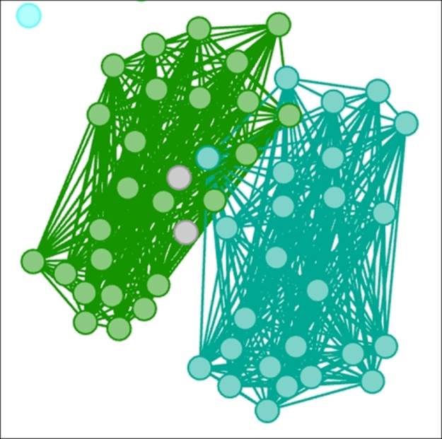
We now have a graph that shows the least connected members of the network, as seen near the perimeter of the graph, and the most highly connected nodes concentrated in the center. The results can be verified in the data laboratory, where we see no nodes with degree values greater than 33 or less than 70. We could follow a similar process using other data attributes such as classname.

I'm sure that you have also thought of some additional applications for complex filters using your own datasets, and it is my hope that these examples will provide both a springboard and reference for some of these processes.

Summary

We covered four main topics in this chapter that will enable you to use Gephi's powerful filtering capabilities to great advantage.

In the first section we explored the purpose of filtering, explaining its benefits and why you should strive to use it for your network analysis in Gephi. We then moved on to describe many of the available filtering functions in Gephi that help you apply good filtering principles.

The last two sections were devoted to help you to apply both simple and complex filters using Gephi. Through multiple examples, we looked at some of the very simple, single filter instances before capping the chapter with some more complex examples using subfilters, intersections, and unions.

In the next chapter, Chapter 6, Graph Statistics, we'll work with many of the available statistical functions available in Gephi and learn how to apply filtering in tandem with network statistics.