Mastering Gephi Network Visualization (2015)
Chapter 6. Graph Statistics
While much of the work we do with graph analysis is visually oriented, there are still some critical ways to assess networks that rely more heavily on calculated measures. These measures can help us to add some hard numbers to our existing graph and begin to compare elements both within a network as well as across networks.
Graph statistics come in many flavors and can be used to assess multiple aspects of a network, giving us additional support beyond the visual analysis we might already have done. In this chapter, we'll take a tour through many of the statistical measures available in Gephi in the following order:
· We'll start with a general overview of graph statistics and learn how and why they are critical to understanding the structure of our network.
· Next, we'll focus on interpreting many of the statistical measures using the Gephi Statistics tab.
· Finally, we'll spend a significant portion of the chapter working with some network data, using the statistics to illustrate structural differences between networks. For this section, we will again use the primary school network data used in Chapter 5, Working with Filters.
Let's begin with an overview of some of the primary methods used within the field, with a focus on those that are available within Gephi.
Overview of graph statistics
There are a number of directions we can head toward when we seek to understand the patterns and behaviors within a network. Here are a few of the key questions we might wish to understand:
· What does the overall structure of the network look like? Is it densely connected, or is the network rather sparse?
· Does our network have a high level of randomness, exemplified by few distinct patterns? Or are there very pronounced groups within the network that exhibit advanced levels of clustering?
· Do we see evidence of high degree hubs in the network, as in the case of the Web, with many smaller nodes surrounding the hubs?
· Are certain nodes critical within the structure of the network, perhaps acting as bridges between otherwise disconnected groups?
Each of these questions (and more) can be answered using graph statistics. Our job in this first section of the chapter is to better acquaint ourselves with which statistics to use and when to measure the various behaviors and structures of a network.
Network measures
Gephi provides many statistics that help us to assess the overall structure of our network, including measures for density, path length, hub detection, and overall connectedness. These measures can provide tangible numbers to help support an initial visual assessment of the network, and can also lead us to explore facets of the network that might have been less than obvious from a visual perspective.
We'll walk through several statistics and explore how you can use them to explore your own networks at a relatively macro level. Later sections will then delve into the patterns within the network, as measured by various centrality and clustering statistics.
Diameter
The concept of diameter in network analysis is very simple; it refers to the maximum number of connections required to traverse the graph. Another way to look at it is knowing how many steps it takes for the two most distant nodes in the network to reach one another. In practice, there will be more than a single pair of nodes that fit this description, but the concept remains the same.
Understanding the diameter of the graph helps us begin to comprehend the structure of a network; a graph with a diameter of three will often be less complex than one with a diameter of seven, although this is not always true. Similarly, if we know that a single node has an eccentricity level of four in a network where the diameter is seven, it lets us know that the node is likely quite central to the network.
Eccentricity
Eccentricity refers to the number of steps required for an individual node to cross the network. This number is limited by the diameter of the graph; for example, a graph with a diameter of seven will have nodes with a maximum eccentricity level of seven.
When used to compare nodes, eccentricity can help provide some context to assess the relative position and influence of nodes within a network. While not a substitute for the various centrality measures, eccentricity can nonetheless provide some clues into the relative importance of individual nodes within the network.
Graph density
Graph density is a measure of the level of connected edges within a network relative to the total possible value and is returned as a decimal value between zero and one. Graphs with values closer to one are typically considered to be dense graphs, while those closer to zero are termed as sparse graphs. What constitutes dense versus sparse will vary depending on the type of network data being studied, so it might not be appropriate to compare numbers between very different network subjects. Nonetheless, this is an important measure to develop an understanding for how an individual network is structured, and might help identify gaps or holes within the graph.
Average path length
The average path length (abbreviated as Avg. Path Length in Gephi) provides a measure of communication efficiency for an entire network, by measuring the shortest possible path between all nodes in the network. An overall number is calculated for the entire network, with lower numbers giving an indication that the network is relatively more efficient, and with high average numbers signifying a relatively inefficient graph for information flow.
This number will necessarily be less than the network diameter, as that value represents the maximum path length between nodes.
Connected components
When we have a network where more than one component exists, the Connected components tool can be used to provide us with a simple read on the number of distinct components within the network. When our network is fully connected, a value of 1 will be returned, so there is little need for this calculation. However, in very large networks it might be difficult to visually determine whether the network is fully connected, so we can use this function to ascertain the number of components.
Erdos number
The original Erdos number definition was based on the number of connections other network researchers had with Paul Erdos, the most prolific (published) mathematician in history, with more than 1,500 papers to his credit. The number that bears his name provides an indication of the collaborative distance between other mathematicians and Erdos. For example, an Erdos number of 1 indicates a direct collaboration with Erdos, while a value of 2 indicates that someone collaborated with one of Erdos' own collaborators, and so on.
In Gephi, this statistic is applied more generally, by specifying a base node (an Erdos proxy), and then determining the Erdos number for all other nodes in the network. Those directly connected to the base node have a value of 1, followed by the nodes which are connected to those with a 1, which have a value of 2, and so on. To work with Erdos numbers in Gephi, be sure to install and activate the Social Network Analysis plugin.
HITS
The Hyperlink-Induced Topic Search (HITS) function is based on the work by Kleinberg, and it calculates two separate values for each node. The first, termed as Authority, provides a measure for how valuable information stored by a particular node is, while theHub number measures the quality of the links to and from that particular node. These measures can help to identify or confirm the roles played by critical members within the network.
Edge betweenness
The edge betweenness statistic provides a glimpse into how often specific edges reside within shortest paths between network nodes. This can help us to illustrate the most efficient paths for traversing a network by identifying the most frequently used paths. As with many of the statistics, the number can be returned in raw nominal form (say 10 or 12), or as a normalized value between zero and one. Normalized values allow us to make comparisons between networks to gauge relative edge betweenness importance levels, while non-normalized numbers are highly dependent on the size and structure of each network.
To work with this measure in Gephi, be certain that you have the Edge Betweenness Metric plugin installed and activated.
Centrality measures
The role of centrality within a network and its member nodes is part of what we generally attempt to understand. There are many ways to measure centrality, each with its own algorithm. Generally speaking, each of these approaches will help us understand a specific type of centrality, as opposed to offering competing versions of the same measurement.
Think of the various ways in which we might wish to understand centrality in a network:
· We might begin by measuring how central a specific node is relative to the entire network. Is the node in question highly connected and centrally positioned within the network, or is it on the fringes with just a few connections? This is probably the first and most obvious of the centrality measures, but there are several other options.
· Is a node surrounded by highly connected neighbors, without necessarily being directly linked to large portions of the network?
· Is a given node most likely to be connected to other key members of a network, thus affirming its status as an important player, or are most of the connections with members on the fringe of the network, thus reducing the influence level?
· Does a node form a bridge between otherwise unconnected portions of the network, even though it might otherwise appear to be unimportant to the network structure? This can be measured by how often a node appears on the shortest path between other nodes.
These are the four critical questions to address when we are applying centrality measures, and each has one or more methods in Gephi to help supply definitive answers. Let's take a look at these methods, first in theory, and then through some actual applications later in the chapter. We will include the standard statistical calculations used for each measure, but it is not critical that you commit these to memory. The definitions are provided for those of you who wish to further understand or explore the mathematical constructs further, but we will not spend additional time on the formulas within this book.
Degree centrality (undirected graphs)
Perhaps the simplest approach to measure centrality is found in this form, where we assess importance through the number of direct connections (degrees) one node has to other nodes. This approach is applicable in undirected networks only, but does have corollary measures (In-degree and Out-degree) designed for directed networks.
The assumption with degree centrality is that the number of connections is a key measure of importance or influence within the network. In an undirected network we do not have the luxury of determining whether one node exerts more or less influence in a relationship; we merely see that they are in fact connected and as such are weighted equally. As anyone familiar with the structure of the Web is aware, this is not always the most accurate way to determine influence, but it likely provides a good proxy for relative importance in a network structure.
Note that there are two ways in which we can measure each of these centrality methods:
· The first, and most obvious way is to use the nominal degree figure, such as 49, 32, or 18 degrees. While this is informative within the context of a single network, it doesn't allow for comparisons between networks. Larger networks are quite likely to have more nodes with a higher degree measure, yet these nodes might not be as important as a node with a lower degree level in a smaller network.
· The second, slightly more informative approach, albeit more complex, is to normalize the number based on the maximum potential degree level. Using the same three numbers, and assuming a network of 200 possible direct connections, we can then calculate the relative centrality of each node. This then provides us with the numbers that are better suited for comparison to other networks, as all nodes will have a decimal value between 0 and 1.
In-degree centrality (directed graphs)
If the graph has directed edges, we have the ability to go beyond the simpler degree measure and split it into In-degree and Out-degree measurements. These two measures can inform us whether a network is highly reciprocal (In-degree and Out-degree measures are quite similar) or not. Referring back to the Web example, a site such as Google has a very high In-degree measure, as millions of external sites link to Google. Most of these sites will have very few inbound links of their own and will therefore have very low levels of In-degree centrality. This will lead us to conclude that the Web is primarily a unidirectional network, characterized by a small proportion of hubs with high levels of In-degree connections, while the bulk of sites are weighted far more heavily to Out-degree links.
Out-degree centrality (directed graphs)
Another important measure for directed graphs is the measure of the number of Out-degrees, defined as connections flowing from a selected node to a range of other network members. We have already noted that a high level of Out-degrees relative to In-degrees will often tell us that a particular node is not thought of as a direct information source. This same node can however provide paths to a variety of critical sources, serving as an information aggregator or hub for others.
Closeness centrality
Closeness centrality represents an interesting case, wherein the selected node might actually be poorly connected in a direct sense, yet is still highly influential due to the proximity of well-connected neighbors. Consider the case of someone who is seen as a gatekeeper to an important and influential person; this individual might have relatively few first degree connections, but is still well positioned due to the presence of a high proportion of highly connected nodes as direct connections.
Eigenvector centrality
When nodes are highly connected to other nodes with high levels of influence, the result will be a high-level of Eigenvector centrality. In this case, it is not simply being connected to many other nodes that is critical, but being connected to the most highly influential nodes is paramount. Google's page rank, the famous algorithm used by Google Search to rank websites in their search engine results is a variation of this approach, taking into consideration the connections between sites and weighting their relative importance in terms of web searches, page hits, and other criteria.
Betweenness centrality
The betweenness centrality presents us with a rather unique case, identifying nodes that might well be poorly connected as defined by other centrality measures. In cases where these nodes offer the most direct path between otherwise disconnected clusters, we have what is often termed as a bridge. Being a bridge is not a necessary precondition to have a high betweenness centrality score, but it is often the case that these nodes will rank as critically important using this measure.
Clustering and neighborhood measures
Another key aspect of network graph structure is the level at which nodes group together into various clusters or groups, defined by some shared characteristics or behaviors. These common characteristics might come about as the result of a wide variety of social or geographic factors, including education levels, race, gender, profession, and so on. Gephi provides a few key statistics to help us assess the relative levels of clustering within a network that we'll discuss in the following sections.
Clustering coefficient
With the Clustering coefficient, Gephi provides us the ability to measure the level at which the nodes are grouped together, as opposed to being equally or randomly connected across the network. Scores on this measure will have an inverse correlation with otherstatistics, including several of the centrality calculations, particularly when we are speaking at the global level (the entire graph). We can also measure this statistic at a local-level, to understand the influence of a single node within its own neighborhood.
This calculation is based on calculating the number of closed triangles (triplets) relative to the potential number of triangles (triplets) available in the network. When we speak of triangles in network graph terminology, we are referencing the connections between the nodes that form complete triangles; in essence, this measures the degree to which your own friends are also friends with one another. In network science language, this could be termed a clique of size 3. High clustering coefficient scores reflect a network where this is most likely true. One might anticipate a high score from tightly knit social groups or clubs (church membership for example), whereas geographically remote networks might be expected to produce lower scores.
At the local level, the measurement determines how likely a single node's neighbors are to form a complete graph (clique). If all possible edge connections are made, the local clustering coefficient would have a score of 1.0, reflecting a graph where all available connections have been created.
Number of triangles
Another way to determine the connectedness and clustering patterns within a network is by measuring the number of triangles present, a measure that provides the nominal count of triangles that are part of the clustering coefficient calculation. This is simply a summation of all possible triplets (connections between three nodes with two or more nodes connected) in an individual node's network, regardless of whether we have a closed triplet (with three edges) or an open triplet (two of three edges are present). To calculate the clustering coefficient, we need to understand what proportions of the triplets are closed (complete).
Modularity
One more approach to measure clustering in a network is through the application of the modularity statistic, which attempts to assess the number of distinct groupings within a network. This can be done simply by using this statistic, or through the use of one of the Gephi plugins geared to parse nodes into distinct groups. The Chinese Clusters tool can be used for this purpose, as well as the MCL, MCODE, and Girvan Newman plugins. The end goal for any of these algorithms is to group nodes based on the strength of their relationships. Nodes that are highly connected are likely to wind up in a common cluster, regardless of which algorithm is employed. Yet each approach will return slightly different results depending on the size and structure of the network as well as the statistical thresholds employed.
Link Communities
The Link Communities function can be used to understand how individual nodes connect to multiple communities or neighborhoods within the graph. This gives us a slightly different view of the network compared to the most clustering or partition approaches, which force each node into a single grouping. In the communities' case, each edge connection is identified with one or more communities, creating a more complex but potentially more insightful mapping of the network and its relationships.
Neighborhood overlap and embeddedness
The idea of embeddedness and overlap are part of a larger area of network analysis termed as social cohesion. While these are not exactly synonymous with traditional clustering, they are certainly related concepts. The basic premise is that rather than neatly defined clusters or partitions, most networks will have nodes with connections into multiple groups or neighborhoods. We can then measure the embeddedness level of specific edges to help determine the neighborhoods where a given node has the strongest associations.
Note
Note that a node can still be connected to other more distant nodes and their respective neighborhoods, but if this is a random or singular connection, the resulting level of embeddedness will be lower.
Interpreting graph statistics
Now that we have discussed all of the measures available in Gephi and provided a brief overview of what they can do, the time has come to understand what the raw numbers signify. Each of these measures provides statistical output that needs to be interpreted in order to understand each and every network and to be able to make accurate comparisons between networks.
Fortunately, many of these measures provide normalized output, that is, values that reside on a zero to one continuum, facilitating easy comparisons between different networks. We'll spend a little time on the interpretation basics before moving on to the actual application of many of these statistics to our working network.
Interpreting network measures
When we are examining the various network statistics in Gephi, our goal is to understand the general structure of the network. There are a few simple questions we need to answer using these functions:
· How large is our network, measured by how many steps it takes for the two most distant nodes to connect to one another?
· On average, is our network closely connected, with perhaps a few outliers, or do a high percentage of the members reside many steps away from other nodes?
· Is the graph relatively dense (that is, many connections between nodes) or would it be considered sparse, with few connections relative to the size of the network?
· Does the network have large hubs with many smaller surrounding nodes, or is there a more random structure to the graph?
· Do we see clearly defined groupings, or is the network highly connected in many directions?
These are all key questions to address as we begin to more fully understand the structure of the network, and they can all be answered using some of the statistical tools we just reviewed.
Before we take this any further, it is critical to understand that all statistical measures are calculated relative to the network we are working on. This means that we cannot literally compare statistics from one network to another, although we might be able to make some of these comparisons in a relative sense. All statistics will be subject to external variables such as the industry or situation being studied, the definition of connectedness (are we measuring collaboration or simple interaction), the time span being studied (if applicable), and a host of other considerations.
So with those caveats in mind, let's move on to a basic understanding of what we are looking for as we interpret each of the available statistics.
One of the simplest measures to understand is diameter, which is merely a measure of the distance between the two most distant nodes in the network. However, even this rudimentary statistic has some subjectivity involved in its interpretation. Let's consider two networks, each with a diameter of six. Simple, right? At least until I inform you that Network A has 200 nodes, while Network B has 2,000. This begins to alter our perception about the structure of each network relative to the other. Network A suddenly seems inefficient compared to Network B, which should at least pique our interest into why these two different size networks require the same number of steps to fully traverse.
Eccentricity is closely related to diameter, as it essentially measures the diameter for each node within the network, versus a single network-based number. Every node in the network (assuming they are all connected) will have a value between 1 and the diameter value, with 1 being highly unlikely. In the case where each of our two networks has a diameter of 6, it would be very interesting to learn how many individual nodes match these criteria. If there are just a few nodes at the edges of the graph with an eccentricity value equal to 6, then there is perhaps little to be gleaned from this information. If, however, 10 percent of nodes in Network A have an eccentricity measure equal to the graph diameter, compared to just 3 percent in Network B, then we can safely assume that the relative structures of the two networks likely differ to a considerable degree.
If we wish to understand the role played by a single node in the network, we can apply the Erdos number calculation to see how all other nodes connect to this single member. In a sense, this is related to the eccentricity calculation we just discussed, although we are now looking at the inverse—how many steps does it take for all other nodes to connect to a single selected member?
The graph density statistic gives us critical feedback on the structure of the graph as measured by the proportion of edge connections relative to the total available number. As you would expect, this will return a value between 0 and 1, with higher values indicative of a dense graph where a majority of available connections have been completed. This is another measure where there is some room for subjective judgment, even though the returned value is based on a mathematical calculation. Take the earlier example of a collaboration network versus a simple interaction (Facebook, for example) network. The collaboration network requires that two or more individuals work together on a paper or project; this is a more challenging criteria compared to the simple acknowledgement that James (and James' friends) is a friend or acquaintance. Therefore, we would anticipate a lower graph density statistic for the collaboration network, given the more demanding connection criteria.
The most appropriate situations to compare graph density measures would be when the types of connections are similar, as in the case of Collaboration Network A versus Collaboration Network B, or Facebook connections versus Twitter connections. Either of these scenarios would furnish us with an apple to apple comparison where the various statistics could be fairly compared.
Average path length can provide insight into the general structure and connectedness of a network. If we reference the average path length for a graph, and find it to be very close to the network diameter, then this is an indication that the graph is inefficient from a communication standpoint. If this is the case, it may well be due to the presence of multiple clusters in the network (homophily) that add friction to the process of traversing the graph.
On the other hand, if the Average Path Length measure is well below the diameter, then it is likely that the network is efficient, and information can easily flow across the graph. We do need to be cautious in making this assessment, particularly if certain paths are heavily dependent on one or more bridge nodes to facilitate connections. In this case, the removal of a single pivotal node may have significant negative consequences on the network as a whole.
The HITS algorithm, as noted earlier, creates both the Authority and Hub statistics, which might or might not provide different values for each node. In the case of our primary school network dataset used in Chapter 5, Working with Filters, identical values are returned using this approach—an indication that no individual member is considered more authoritative than any other. In other words, the weighting is equal for all nodes, leading to values that are aligned with the hub statistics. If we had a directed network, the results would almost certainly be different. We still see differentiation within the hub statistic—a finding that is consistent with the degree measure produced earlier—but we have no way of determining the direction of the links; so no additional value comes out of the Authority number.
HITS is similar to the PageRank method for assessing web pages, with higher authority scores indicative of a page that is linked into by many hubs (In-degree connections), while the hub calculation is based on the number of outbound links (Out-degree connections).
Edge betweenness is an approach that helps to sort out the paths that are most often taken to minimize travel across the network. In the normalized version, this measure will reside somewhere between 0 and 1, with a score of 1 indicating that all nodes must travel via that particular edge to reach a desired node or nodes. Conversely, scores near 0 signify that there are other more efficient paths to use to make the shortest journey between two or more points. In the case where a small number of paths carry very high values (that is near 1), there is a risk that if these connections are lost, the network will become more fragmented and communications across the graph will suffer.
Now that we have a more complete understanding of how to interpret and apply generalized graph statistics, we can move onto the various node-based centrality measures and understand how to interpret their output.
Interpreting centrality statistics
Centrality statistics provide the framework to compare the roles played by various nodes within a single network. Given that every node is resident in the same graph, we are able to judge these statistics on equal footing, as all nodes (at least in theory) have the same opportunities. In practice, as we have already seen from our school network, some members might be better positioned than others based on constructs such as grade level, physical location, and so on. If these structures influence the network significantly, we still have the ability to compare results within smaller groups such as individual classes.
Let's take a look at how we might construe the meaning of the statistical results provided by each of the centrality algorithms.
Degree centrality
Degree centrality, as noted earlier, is the simplest of the centrality measures, as it calculates a result based only on the number of connections possessed by a given node. This number does not inform us about the strength of each connection, nor does it tell us the importance of any connections. So when we look at results and see that Node 1551 has 98 direct connections, and Node 1609 has merely 18, we can probably assume that this indicates a dramatic difference in their respective levels of influence in the network. However, in cases where the difference is of a much lower magnitude, we would not be so comfortable making this claim and would certainly want to support it through some of the more sophisticated measures to follow.
In-degree centrality
When we have a directed graph, In-degree centrality provides a more robust measure of influence compared to a simple degree measure. This measure tells us how likely other nodes are to seek out a single node, whatever the reason might be—charisma, money, perceived influence, knowledge, or some other attribute that makes this member an attractive target for others. Let's assume from our earlier case that we have a directed graph, and we discover that Node 1551 has an In-degree measure of just 18 (implying an Out-degree number equal to 80). Let's also assume that Node 1552, with a total of 90 degrees, has an In-degree value of 50. Now who seems to play a more influential role in the network? A simple undirected degree measure would have told us that 1551 was marginally more important, while our In-degree number portrays a vastly different story. In this case, 1551 would appear to be a social butterfly who seeks out others, while 1552 is perceived as someone who provides greater influence, power, or prestige.
Out-degree centrality
Out-degree centrality, as we just touched on, might well indicate someone who reaches out to others for more information, influence, or prestige; or in the case of the Web, it could be an indication that many small sites have high connection levels to hubs such as Google or Yahoo!. This is especially the case when there is a significant imbalance between the Out-degree and In-degree measures. Certainly, it is possible for individuals to have relatively even profiles in this respect, although this is generally not the case when networks are dominated by a small number of hubs, be they individuals, websites, or some other entities.
Closeness centrality
With Closeness centrality, we begin moving toward a more sophisticated measurement of centrality; in this case defined by the effort required (as measured by path length) to reach all other nodes in the network. As noted earlier, we might well have a number of graph members who score low on other measures such as degree centrality, but who still exercise influence based on their position within the network. It is often the case that a single node scores highly on each of these measures; if an individual has enough degree connections, she/he will likely have fewer long path connections to other nodes, resulting in a lower (that is, more connected) score on this statistic.
In terms of output, each node will have a measure higher than 1, with lower values indicating greater centrality. Members of the network located at the outer edges are highly likely to have high relative scores, as they require more steps to reach all other nodes in the network. A final note on Closeness centrality is that our network must be completely connected in order to run this measure, otherwise we get an infinite result.
Eigenvector centrality
Eigenvector centrality takes Closeness centrality a step further. Instead of being most concerned by the number of steps required to reach all other members of the network, our focus is on the importance of the connections. This is measured by understanding whether individual nodes have a high proportion of their connections to influential members, which boosts their own standing. This is calculated on a 0 to 1 continuum, with values near 1 indicating the highest levels of centrality. In our school classroom network, values range from 0.1 to 1, indicating vastly different levels of influence within the network.
Eigenvector centrality is likely to show a positive correlation with Degree centrality and Closeness centrality, although the relative correlations will of course change depending on the network structure.
Betweenness centrality
Betweenness centrality plays a unique role in understanding how information, influence, and even diseases flow within networks. Unlike the other centrality measures, which are largely predicated on direct connections and/or proximity to others with many connections, betweenness measures how important an individual node is for others traversing the network. Specifically, this measure tells us how often a given node lies on the shortest path between two other nodes.
It is quite possible, and often likely, that a member with a very high betweenness centrality score has very low numbers on all of the other centrality calculations. This will be highly dependent on the network structure and is far more likely to be true in networks with higher levels of clustering.
From here, let's transition to a discussion on the meanings of the various clustering statistics, and how we can develop a better understanding of the aggregation patterns within the network. These measures will help to bridge the gap between statistics that examine the network in its entirety and the centrality calculations, which were focused on the role of individual members within the network.
Interpreting clustering statistics
Clustering statistics are crucial to our understanding and interpretation of network behavior, and specifically, how individual nodes interact and form groups, or clusters. This is the third and final series of graph statistics that begins with the concept of overall network structure as embodied by measures such as diameter, path length, eccentricity, and edge betweenness. Our second series of statistics was focused on centrality, and how individual nodes are related to the network as a whole. When we look at clustering behaviors, we are synthesizing the first two series through the study of how individual nodes work together to shape the internal structure of the network. These measures will help close the loop to understand why certain networks have very high (or low) diameters relative to the number of members, and help us to understand how individual nodes manifest high (or low) centrality scores.
We'll begin with a discussion of how to interpret the clustering coefficient score, followed by brief overviews to understand triangles, modularity, Link Communities, and finally embeddedness.
Interpreting clustering coefficients
The global clustering coefficient is based on the concept of triplets: three nodes often in close proximity to one another, connected by two or three edges. In the case of two connections, the triplet is referred to as an open triplet, while if all three nodes are connected with one another, we have a closed triplet, also referred to as a triangle. The derived statistic is simply calculated by dividing the number of closed triplets by the total number of triplets (open and closed), resulting in a coefficient value between 0 and 1.
An interesting observation can be made about clustering coefficients—they are often inversely correlated to the number of degree connections possessed by a single node. Part of this is easily explained—those nodes with many connections spanning a network are likely connected with many others less likely to have the same behavior (most networks show a wide degree range from low to high). This is certainly the case in our school network, where the most highly connected members have rather low clustering coefficients, while those nodes that tend to stay closer to home with their links sport much higher values. The idea of having your own friends connect to one another (thus forming closed triplets) is more likely to happen in smaller, more cohesive groups, and this is ably demonstrated by the school network example.
Number of triangles
The Number of triangles statistic is simply a nominal count of all the available triangles generated by a node's degree connections. As you might have anticipated, this is strongly positively correlated to the number of degree connections, although the literal rank order might change slightly. Used in tandem with the clustering coefficient value, we can back into the number of closed triplets each node has in their personal network; just allow some rounding error differences.
Modularity
The Modularity statistic places individual nodes into an aggregated group or cluster based on shared characteristics. This is a simpler approach compared to plugins expressly designed for clustering and partitioning, but it can nonetheless help in understanding the network and provides a very easy means to do so when combined with filtering methods. Output for this function is simply an integer value starting at 0.
Link Communities
With the Link Communities statistic, we can begin to understand deeper levels within the network that might go undetected if we rely on traditional clustering or partitioning approaches. This statistic will group edges into communities based on similar patterns, applying a single number to every edge in the network. These communities can encompass a single edge or can be composed of dozens of edges that follow similar paths.
Embeddedness
Embeddedness refers to the level at which specific edges tie nodes into neighborhoods across the network. If a given edge connects two nodes across the network in a solitary fashion, then we will expect the embeddedness score to be quite low, perhaps approaching zero. This suggests that these two nodes have relatively little in common, despite their direct connection, which might be simply incidental. The fact that the two nodes have been positioned far apart from one another by a layout algorithm confirms this belief.
Higher embeddedness scores can help direct us toward an understanding of secondary neighborhoods that a given node is linked with, which might be far less evident through a simple inspection of the network layout. We would still anticipate the highest scores to be strongly correlated to the close physical proximity of similar nodes; however, some moderately high scores might point us to other associations or neighborhoods that are important to an individual node.
Application of statistical measures
In this final section of the chapter, we're going to apply many of the statistics we've just reviewed to our school classroom data and begin to gain a greater understanding of the network beyond our earlier visual assessments. Even better, we will use the power of filtering in tandem with the graph statistics to begin using Gephi in an even more sophisticated fashion. We'll start this section with some fairly straightforward examples, and then move on to more complex analysis using the available filtering options.
Basic statistical applications
We're going to work once again with the primary school dataset as we will illustrate the practical application of many of these statistics. We'll proceed in the following order:
· The first section will apply some of the network-oriented measures that will inform us about the general structure of the graph
· Our second section will view several of the centrality statistics and compare how individual nodes are classified
· We will close out by taking a look at a few of the clustering statistics in order to gain a better understanding of how individual nodes form groups based on their behaviors and location within the graph
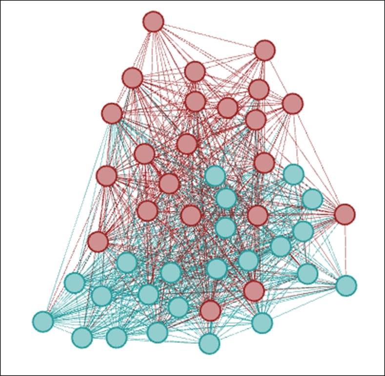
Let's begin by checking out a few of the network-based statistical measures, and what they tell us about our primary school data. We'll work through each of these statistics by providing the calculated values from the school network graph, and follow with discussions on the overall meaning of each measure. Before we begin, it might be helpful to see the network as follows:
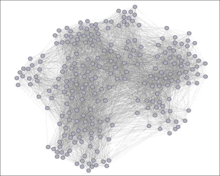
Primary school network
Network statistics
The several measures discussed in this section will provide a lens into the general structure of the network—its size, density, and efficiency will be examined as ways of understanding the composition of the graph. These statistics will help lay the groundwork for the more detailed centrality and clustering measures to follow. Remember that each of these statistics (and many others) can be found in the Statistics tab within Gephi. For most, all that is necessary is to click on the Run button. For a few others, you will need to specify whether your network is directed or undirected.
Let's see what results we get for some of the critical network statistics. You should be able to easily validate these numbers in your own Gephi instance.
Network diameter
The maximum steps required to cross the network is three, which would seem to indicate a network without a lot of clustering. This seems to be a fairly low value relative to the total number of nodes (236).
Eccentricity
About 20 percent of the nodes have an eccentricity value of 2, with the remaining 80 percent requiring three steps to reach the furthest member of the graph. This provides further confirmation that this network is relatively evenly distributed and easily traversed by all nodes. We do not have any outliers at the fringes of the network who require four or five steps to cross the graph (this would require a higher network diameter, of course).
Graph density
About 21 percent of nodes are connected with one another, based on the output value of 0.213. This is neither an exceptionally high number, nor could it be considered very low. If we reflect on the parameters of this network (grade levels, individual classes), the number appears to make sense in its context. The next step would be to compare this with the same measure from a similar network to judge whether this value is within an expected range (as it seems), or if this network is typically well connected or poorly connected.
Average path length
It takes nodes close to two steps (1.86) on average to reach any other node in the network. This feels like a reasonable number given the prior measures we have discussed. If our graph density figure was considerably higher, we would then anticipate a lower average path length, as a higher proportion of members would have first degree connections.
Edge betweenness
As expected in a well-connected network, there are often multiple paths available to reach specific nodes, resulting in only a few edges with very high values; for instance, 97 percent of all edges have values below 0.5, with the range running between 0.34 and 1.0 The literal translation is that there are just 3 percent of cases where more than 50 percent of all nodes must travel along a single path to reach another node most efficiently (that is, shortest path). This informs us that we have a very robust network for information flow, and that even if a number of links were broken, the network would still be well-connected and efficient.
So what have we learned about the structure of this particular network?
· Overall, it seems safe to assume that this is generally a tightly knit network with minimal variation, as determined by eccentricity levels
· The network appears to be well-connected judging from the graph density measure, but it does not seem to be especially dense
Next, we'll look at a handful of centrality statistics from the same network, and determine what sort of story they are telling us about the behavior patterns of individual nodes inside the graph.
Centrality statistics
We previously talked about the use of centrality statistics for understanding the role played by each member of the network. In this section, we will also see how these measures help to define aggregate patterns within the graph and begin to understand how these individuals interact with one another. Our analysis will be based on four key centrality approaches: degree, closeness, eigenvector, and betweenness.
Degree centrality
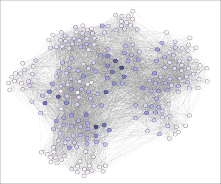
There is a considerable variation in the degree ranges within this network (from 18 through 98), as is the case in the majority of network graphs. This is not an extreme variation in the sense of measuring nodes on the Web, but given the total potential number of degrees (n-1 = 235), it does represent a significant variance. To help illustrate these differences, let's have a look at a graph where we have colored the nodes based on degree level—darker colors being indicative of higher degree counts:
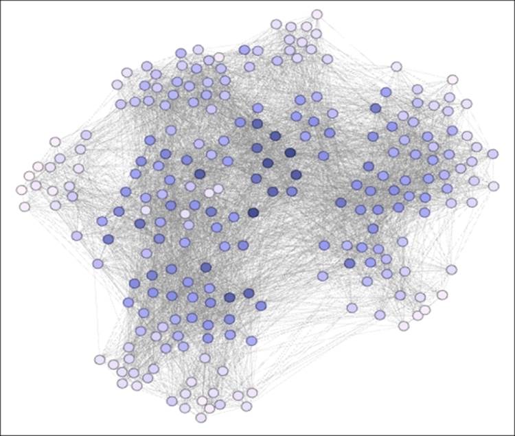
Degree centrality expressed using node coloring
We can now see how the high degree nodes tend toward the center of the graph, while those with low degree values are forced to the perimeter; a typical pattern for many layout algorithms. It is also evident that many of the high degree members are in close proximity to one another, an observation which will prove consistent with the lack of significant clustering in this network. This fact will also influence some of the other centrality measures.
Closeness centrality
This is a much tighter distribution (1.583 through 2.209) than we saw for degrees, largely attributable to the generally close-knit structure of this network. As you can recall, the eccentricity level for all nodes was either 2 or (mostly) 3, an indication that there are no far-flung outliers residing at a great distance from the center of the graph. In cases where there was a greater distribution of eccentricity, we would anticipate a more dispersed distribution of values for this statistic. Visually, this is what we see, again coloring the values based on the statistic, with higher closeness scores (that is, greater distance) indicated by darker nodes:
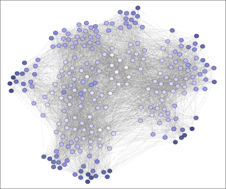
Closeness centrality expressed using node coloring
Remember that this is a sort of inverse measure—higher values indicate more distant levels of proximity to other members of the network. So the same nodes that had fewer direct connections are also associated with higher closeness measurements, which should come as no surprise. Those in the center of the graph can more easily travel to all other nodes in the network (on average), while members on the perimeter cannot do so quite so easily.
Eigenvector centrality
In contrast to the narrowly distributed values within the closeness centrality statistic, we see a far greater range for the eigenvector measurement (0.108 through 1). Now we are attempting to understand the relative importance of connections to gauge whether influential members are likely to be connected with other members of similar standing. Likewise, this measure will tell us whether nodes with lower influence are more likely to be connected with their peers. In this case, both of these patterns appear to be true, giving us a wide range of values. Our example looks like this:
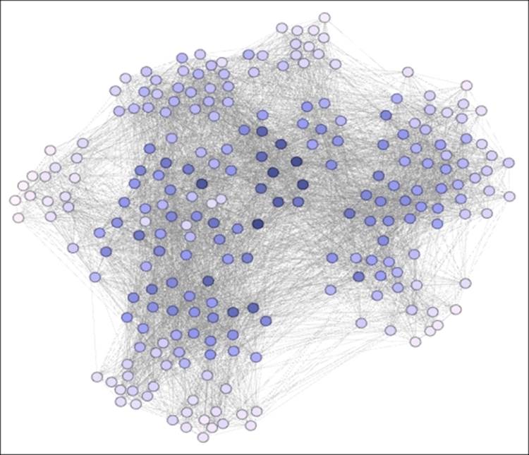
Eigenvector centrality expressed using node coloring
Here, we have a diagram that resembles, but differs slightly from the degree centrality image shown a moment ago. As expected, the higher levels of centrality are concentrated in the center of the graph, with a general progression toward lower levels as we approach the perimeter. Influential nodes are surrounded by other influential nodes, with the inverse also true, that is, low degree members are largely enmeshed with similarly behaving nodes.
Betweenness centrality
There is a rather large spread in betweenness centrality from top to bottom (2.7 to 396.7), with a few nodes having values near zero located around the perimeter of the network. At the other extreme is a total of 8 nodes with betweenness measures of 300 or greater. These members are important players that help to connect diverse portions of the network, although we don't have any that fill the classic role of a bridge between clusters. A view of this statistic seems to confirm what we have already learned about the network:
Betweenness centrality expressed using node coloring
As expected, nodes at the perimeter have very low betweenness scores—there is nowhere to go that requires traveling through these members. However, we can detect a handful of critical members that facilitate network traversal, and notice how they are spread out to a much greater degree than we saw for some of the other measures. This is actually quite logical, as it would make little functional sense to have two nodes with very high betweenness properties sitting adjacent to one another; this would be highly redundant. Instead, we can see a more scattered pattern with one or two high scoring nodes strategically located within the graph, which help to create a more efficient network.
Based on these statistics, we can safely conclude the following:
· There is a high level of differentiation across individual nodes, as shown by the variance in degree level
· The most highly connected nodes tend to associate with one another, while lower degree members primarily link to similar sorts of nodes
· There is considerable differentiation in betweenness centrality, even though the network does not require bridge nodes
Our third and final section will examine a few of the clustering measures available in the Statistics tab, and what they can tell us about the behavior patterns within this network.
Clustering statistics
Our aim in interpreting the clustering statistics is to comprehend larger behaviors taking place within the network, to see if there are identifiable patterns that tell a significant story. Conversely, the lack of any evident clustering behaviors can also tell a story about the network. We'll analyze five key statistics in the context of our school network to unearth any patterns, beginning with the clustering coefficient.
Clustering coefficient
As we discussed earlier, this is a measure that determines the percentage of available triplets that are fully closed. The statistical measures are 0.502 for the network, and 0.338 to 0.877 for individual nodes. In the case of our school network, the total network number is almost exactly half closed, with the remaining 50 percent still open—two of three edges are connected, but the third edge is missing.
Is this a high or low number? Again, this is somewhat subjective as well as dependent on the individual network, but it does seem to be a rather high figure. If we reflect back to what this network is measuring, this should not come as a complete surprise; we are not looking at long-term relationships or collaborations, but simply interactions between individuals within and across classrooms. The number will almost certainly grow if we restrict it to a single grade level or classroom, as it will reflect the proximity of members throughout the course of a day.
When we examine patterns at the individual member level, we see a wide range from less than 35 percent up to nearly 90 percent of all triplets being closed. Remember that this statistic is inversely correlated to the number of degrees and it begins to make sense. Nodes with relatively few connections are considerably more likely to have a high percentage of closed triplets, while the lowest coefficients come from some of the most aggressively connected members of the network.
Number of triangles
There is a very wide range of triangles from the minimum (96) to maximum (1,616) number of triangles at the node level. At first, this variance seems extreme, but if we step back and look at a couple of other statistics, these numbers make complete sense. First, consider that our degree ranges ran from 18 to 98, and second, remember that many of the most popular nodes are connected with one another (the same is true for the least popular ones). This creates a geometric effect that favors the most highly connected nodes, at least in terms of the number of available triplets. However, as we learned from the clustering coefficient figures, a majority of these triangles will remain incomplete.
Modularity
The modularity statistic splits this graph into five distinct clusters, numbered from 0 through 4. Doing some simple math tells us that each cluster will average close to 50 nodes. This might be satisfactory for our purpose, or if we need further splits, we can employ one of the dedicated clustering algorithms. A quick way to determine if this number is adequate is to color the graph using the modularity class, as we have previously done with the centrality measures.
Link Communities
This network has many Link Communities ranging in size from a single edge to well over 100 edges. What this tells us is not clear from a purely statistical viewpoint, but it can help us decipher interactions between multiple nodes, as defined by their connecting edges. In fact, the two most prominent communities in this graph account for greater than 20 percent of all connections, providing a new insight about the common behaviors that might be less clear if we rely solely on node-based statistics.
Embeddedness
Our final clustering-oriented statistic to measure is embeddedness, which will aid us in understanding the depth at which nodes are affiliated with specific groupings. This measure can help explain how specific nodes or groups of nodes cooperate with one another beyond simply being superficially connected. In our school network, we have an average embeddedness level of 24.6 with individual edge values ranging from 0 to 64. If we examine the data further, it tells us that those edges with very low counts (infrequent interactions) are found at the lowest embeddedness levels; conversely, the highest scores typically correspond to frequent interactions between two nodes.
In the first case, this would represent the sort of superficial connection just referenced; perhaps this contact was random or incidental to a certain time and space. As the frequency of contacts between two parties grows (and with it, the embeddedness score) we can be fairly certain that this is not a random pattern, but something more purposeful and structured.
Now that you have learned how to work with a variety of useful statistics, it's time to take them to the next level by combining them with the powerful filtering capabilities in Gephi. We'll look at a number of graphs in this section so that you get a feel of both, the visual output of the various statistics as well as the multiplicative power delivered by the filtering capabilities of Gephi.
Filtering using graph statistics
We spent a lot of time with filtering in the previous chapter prior to diving into graph statistics. Now we have an opportunity to combine these two powerful features in Gephi, as we can employ most of the statistical measures we have just reviewed as filters to help refine our graph output. This capability gives us considerable power to learn more about our network and drive attention to the most important aspects of the graph. We can also probe to understand the statistical variation within the network which might provide some surprises that would otherwise go unnoticed.
We'll use multiple graphs in this section to help illustrate the impact of combining statistics with filtering. So let's begin by working with some rather simple examples before stepping up the complexity level and showing some of the impressive capabilities of Gephi.
Let's begin with a simple case where we wish to focus our attention on only those nodes that meet a specified betweenness criteria; so we can better understand which nodes are most critical to connect sections of the network. If you recall, our betweenness levels ran from near zero all the way to nearly 400. We're going to follow a few steps to set a filter for only those nodes with betweenness levels above 250. While this number is slightly arbitrary, it is designed to identify the top 5 percent to 10 percent of the influential nodes. Refer to the paper Identifying High Betweenness Centrality Nodes in Large Social Networks, Nicolas Kourtellis et al, 2014, for more insight into identifying the impact of betweenness centrality.
This should give us a good sense for which members are most adept at connecting other nodes. Perform the following steps:
1. Open the Filters tab in the Gephi workspace.
2. Navigate to the Attributes | Range | Betweenness Centrality attribute.
3. Drag the filter down to the Queries area.
4. Set the lower range to 250 using the slider control or type the value manually.
5. Click on Select and then Filter to get the results.
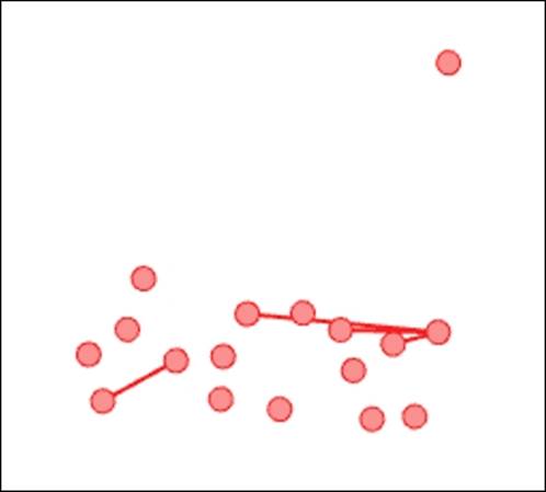
The original network of 236 nodes has now been dramatically reduced, as shown in the following graph:
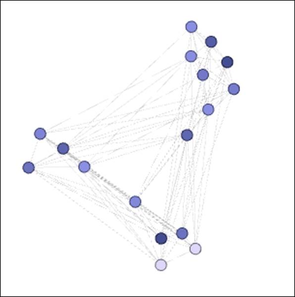
Nodes with betweenness centrality levels greater than 250
We now see the 17 most influential modes in terms of their ability to connect to others in the network. We can of course manipulate the filter to further reduce this group by raising the threshold, or to expand it by reducing the lower bound of the filter.
If you have been working along with these examples, you will have noticed many other statistics that are now available for filtering purposes. In addition to the various centrality measures, we now have the ability to look at hubs, triangles, neighborhoods, eccentricity, embeddedness, and communities, among others. We can also begin to apply some of the more advanced filtering techniques we worked with in the last chapter, giving us incredible power over the network. Let's take a look at a few of these possibilities.
We'll begin by merging the betweenness measure with a specific classname in order to understand which members are most likely to be the bridges within a given class. We're going to assume that you have already applied the previous filter. If not, you can start by following the last process of setting the Range filter using betweenness centrality:
1. Set the lower bound of the range to 150.
2. Run the Select and Filter processes to verify the new setting.
3. Navigate to the Attributes | Partition | classname variable.
4. Drag this filter to the Queries window, as a separate filter and not a subfilter.
5. Click on the 2B option in the Partition Settings window.
6. Go to the Operator | INTERSECTION filter.
7. Drag this to the Queries window, again as a separate filter.
8. Move each of the prior filters under the INTERSECTION query as separate subfilters. Repeat steps 3 and 4 by dragging the classname filter to the subfilter area of the original classname filter.
9. Apply the filter by running the Select and Filter processes.
We now have a new result that has merged our two filters by requiring a betweenness centrality of at least 150 combined with membership in classname 2B. I took the liberty of adding node labels, so we can see who these individuals are:
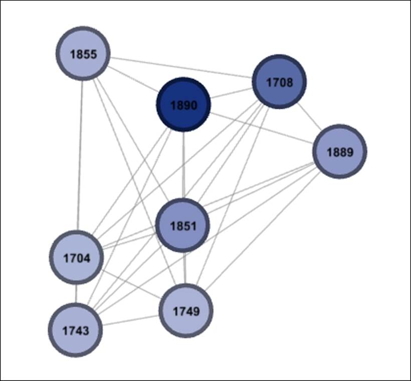
Intersection of betweenness and classname filters
If you wish to see additional details, simply navigate to Data Laboratory, which will now show only the results for these 8 nodes. Of course, if you wish to reduce this set, or apply the logic to a different classname, then simply adjust the filters we just created. Be sure that your two classname filters match; otherwise you'll be staring at a blank graph window.
While it might seem that setting these filters requires a lot of steps, it really becomes much simpler the more you go through the process. However, a great way to avoid having to repeat all of these steps is to save your queries after they have been adjusted to your satisfaction.
To do this, perform the following steps:
1. Go to the top of the query (the INTERSECTION level in this case) and right-click on it.
2. Select the Save option, and your complete set of filters will be saved into the Saved queries folder.
3. You can test that the save process works by removing the existing filters from the Queries window, followed by dragging the saved query to the vacated space. Apply the usual select and filter steps, and you will see your expected results in the graph window.
Saving your complex filters can be a great way to save time and effort and will allow you to create many queries that can then be easily substituted for one another.
It is time to move on to our next example. This time around, we'll work with some of the clustering output we've already created using the statistical functions. Here's our scenario we would like to answer. We already know that the network is divided into specific classnames, based on the grade levels and assigned classrooms within the school. What we really want to know is whether this paints an accurate picture of how the school functions during a typical day. Do students tend to associate with others in their classrooms, or at least within the same grade level, or are there informal structures that are better predictors of information flow? To answer this, we will utilize the Modularity Class calculated earlier and intersect those values with some of the more formal attributes such as classname.
Let's take the following steps to construct our filter to test the above questions:
1. Navigate to Attributes | Partition | Modularity Class in the Filters tab.
2. Select and drag this filter to the Queries window.
3. Set Modularity Class to 3 by clicking on the color rectangle next to the 3 value.
4. Now create the classname filter, as we did in the prior example by going to Attributes | Partition | classname and dragging that selection to the Queries window above the modularity filter.
5. Select the 1B, 2B, 3B, 4B, and 5B values by clicking on the corresponding rectangles.
6. Create a subfilter within the classname filter by repeating steps 4 and 5.
7. Drag an intersection operator to the Queries window and then add each of the prior queries (modularity and filter) as subfilters within the intersection filter.
8. Run the Select and Filter processes.
Our theory here is to see whether we will find evidence of multiple classes from the B portion of the classnames winding up within a single modularity. If this is true, then we might regard the modularity value as being more predictive of network behavior than the more formal constructs of grade levels and classnames. Let's find out whether this is true by looking at our filtered graph, which we'll color by classname using the Partition tab and classname field:
Intersection of modularity and classname for B classes
Our returned graph shows a single color corresponding to classname 5B. This means that not a single member from 1B, 2B, 3B, or 4B is classified within this modularity class. It looks like classname might in fact provide a strong proxy for network behavior. What happens if we expand our filter to include classname 5A to see if any of these students wind up in the same modularity class? Let's have a look:
Intersection of modularity and classname with addition of 5A
We now see that Modularity Class 3 also contains many members from 5A as well as 5B, an indication that the grade level is in fact a very strong predictor of network behavior, at least based on how the modularity algorithm has classified the network.
Our next example will filter on a combination of nodes and edges to get to our desired result. Suppose we want to understand the relationships within a modularity class for nodes that score high on the hub measure we saw earlier in the chapter. We can do this by using a partition filter for the modularity class and a range filter to set the hub threshold. Now what if we wanted to also limit the number of edges based on a certain threshold, such as the embeddedness statistic? We can do this as well using the range filter, so we'll wind up with a query that filters both nodes and edges all at once.
Here are the steps to follow:
1. Navigate to the Equal | Modularity Class filter and drag it to the Queries window.
2. Set the value equal to 2.
3. Repeat this process as a subfilter to the original modularity filter and set it 2 for the second time.
4. Navigate to the Range | Hub filter and drag it to the Queries window; be sure it is a standalone filter rather than a subfilter.
5. Set the minimum range level to 0.005.
6. Go to the Range | Embeddedness filter and drag it to the Queries window, again as a standalone filter.
7. Set the embeddedness minimum value to 50 using the slider control or by typing a text value.
8. Add an INTERSECTION operator to the Queries window.
9. Now drag each of the three queries to the subfilter area of the INTERSECTION filter.
10. Run the Select and Filter processes to apply the entire filter.
We now have a custom view that shows only nodes from Modularity Class 2, with a Hub value of greater than 0.005, and with edge embeddedness levels greater than 50. Here's our result:
Intersection of node and edge filters
These examples scratched the surface of what can be done by filtering using statistical measures. There are many other conditions and combinations which you can apply to your own networks, perhaps using these instances as templates for knowing how to proceed. While we noted that filtering on these attributes is not always easy or intuitive, I believe you will come to appreciate the power that statistics and filters deliver to your own network analysis.
Summary
In this chapter, we covered many of the most critical graph statistics, dividing them into three basic categories: network, centrality, and clustering measures. In the first section, we walked through brief overviews of what each of these statistics can provide for analyzing networks in Gephi.
The second section focused on the interpretation of each of these statistics, when and where they are useful, and what sort of numerical output to anticipate in each case. This was followed by examples of actual applications of these statistics using our primary school network graph.
We closed the chapter with multiple examples showing how graph statistics and filtering can be used together for advanced analysis of any network graph. These examples provided step-by-step instructions that can serve as templates for additional statistical filtering.
We'll now move on to Chapter 7, Segmenting and Partitioning a Graph, where we will explore the multiple methods to improve our graph by identifying common node characteristics.
All materials on the site are licensed Creative Commons Attribution-Sharealike 3.0 Unported CC BY-SA 3.0 & GNU Free Documentation License (GFDL)
If you are the copyright holder of any material contained on our site and intend to remove it, please contact our site administrator for approval.
© 2016-2026 All site design rights belong to S.Y.A.