Hadoop Essentials (2015)
Chapter 5. Storage Component – HBase
One of the most important components of the Hadoop ecosystem is HBase, which utilizes HDFS very efficiently and can store, manage, and process data at a much better performing scale. NoSQL is emerging, and there is a lot of attention towards different implementations and solutions in Big Data problem solving space. HBase is a NoSQL database which can process the data over and above HDFS to achieve very good performance with optimization, scalability, and manageability. In Hadoop, HDFS is very good as storage for the WORM (Write Once Read Many) paradigm where data is not updated. In many scenarios, the requirements would be updating, ad hoc analysis or random reads. In HDFS, processing these requirements is not very efficient as updating a record in a file is not possible; HDFS has to delete and rewrite the whole file which is resource, memory and I/O intensive. But HBase can manage such processing efficiently in a huge volume of random read and writes with a near optimal performance.
In this chapter, we will cover the needs and the necessity of HBase and its features, architecture, and design. We will also delve into the data models and schema design, the components of HBase, the read and write pipeline, and some examples.
An Overview of HBase
HBase is designed based on a Google white paper, Big Table: A Distributed Storage System for Structured Data and defined as a sparse, distributed, persistent multidimensional sorted map. HBase is a columnar and partition oriented database, but is stored in key value pair of data. I know it's confusing and tricky, so let's look at the terms again in detail.
· Sparse: HBase is columnar and partition oriented. Usually, a record may have many columns and many of them may have null data, or the values may be repeated. HBase can efficiently and effectively save the space in sparse data.
· Distributed: Data is stored in multiple nodes, scattered across the cluster.
· Persistent: Data is written and saved in the cluster.
· Multidimensional: A row can have multiple versions or timestamps of values.
· Map: Key-Value Pair links the data structure to store the data.
· Sorted: The Key in the structure is stored in a sorted order for faster read and write optimization.
The HBase Data Model, as we will see, is very flexible and can be tuned for many Big Data use cases. As with every technology, HBase performs very well in some use cases, but may not be advised in others. The following are the cases where HBase performs well:
· Need of real-time random read/write on a high scale
· Variable Schema: columns can be added or removed at runtime
· Many columns of the datasets are sparse
· Key based retrieval and auto sharding is required
· Need of consistency more than availability
· Data or tables have to be denormalized for better performance
Advantages of HBase
HBase has good number of benefits and is a good solution in many use cases. Let us check some of the advantages of HBase:
· Random and consistent Reads/Writes access in high volume request
· Auto failover and reliability
· Flexible, column-based multidimensional map structure
· Variable Schema: columns can be added and removed dynamically
· Integration with Java client, Thrift and REST APIs
· MapReduce and Hive/Pig integration
· Auto Partitioning and sharding
· Low latency access to data
· BlockCache and Bloom filters for query optimization
· HBase allows data compression and is ideal for sparse data
The Architecture of HBase
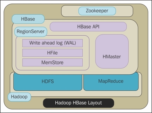
HBase is column-oriented by design, where HBase tables are stored in ColumnFamilies and each ColumnFamily can have multiple columns. A ColumnFamily's data are stored in multiple files in multiple Regions where a Region holds the data for a particular range of row keys. To manage Regions, MasterServer assigns multiple Regions to a RegionServer. The flexibility in the design of HBase is due to the flexible RegionServers and Regions, and is controlled by a single MasterServer. HBase Architecture uses Zookeeper to manage the coordination and resource management aspects which are needed to be highly available in a distributed environment. Data management in HBase is efficiently carried out by the splitting and compaction processes carried out in Regions to optimize the data for high volume reading and writing. For processing a high volume of write requests, we have two levels of Cache WAL in RegionServer and MemStore in Regions. If the data for a particular range or row key present in a Region grows larger than the threshold, then the Regions are split to utilize the cluster. Data is merged and compacted using the compaction process. Data recovery is managed using WAL as it holds all the non-persistent edit data.
The HBase architecture emphasizes on scalable concurrent reads and consistent writes. The key to designing an HBase is based on providing high performing and scalable reads and consistent multiple writes. HBase uses the following components which we will discuss later:
· MasterServer
· RegionServer
· Region
· Zookeeper
Lets have a look at the following figure:
MasterServer
MasterServer is the administrator and at a point of time, there can be only one Master in HBase. It is responsible for the following:
· Cluster monitoring and management
· Assigning Regions to RegionServers
· Failover and load balancing by re-assigning the Regions
RegionServer
RegionServers are identified by the MasterServer, which assigns Regions to a RegionServer. RegionServer runs on a DataNode and performs the following activities:
· Managing the Regions in coordination with the master
· Data splitting in the Regions
· Coordinating and serving the read/write
Along with managing the Regions, RegionServer has the following components or data structures:
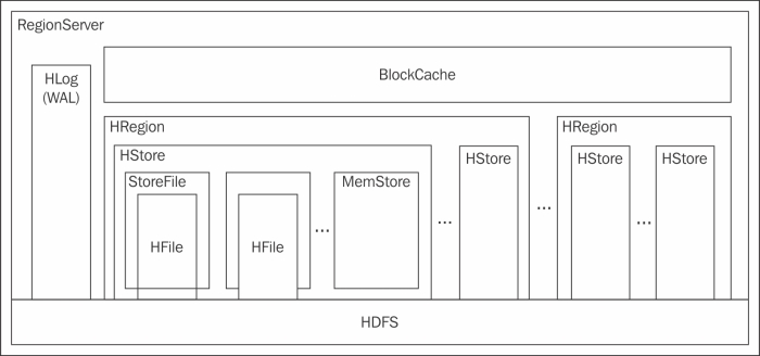
WAL
The data for Write in HBase is first kept in WAL and then put in MemStore. MemStore doesn't persist the data, so if a Region becomes unavailable, the data could get lost. WAL is extremely important in case of any crash, or to recover the data present in the MemStore of a Region which is not responding. WAL holds all the data present in the MemStore of the Regions managed by the RegionServer. When the data is flushed from MemStore and persisted as HFile, the data is removed from WAL too. The acknowledgement of a successful Write is given to the client, only after the data is written in WAL successfully.
BlockCache
HBase caches the data block in BlockCache in each RegionServer when it is read from HDFS for future requests for the block, which optimizes random Reads in HBase. BlockCache works as an in-memory distributed cache. It is an interface and its default implementation is LruBlockCache which is based on the last recently used algorithm cache. In a newer version of HBase, we can use SlabCache and BucketCache implementations. We will discuss all the three implementations in the upcoming sections.
LRUBlockCache
The data blocks are cached in a JVM heap which has three areas based on the access request, that is, single, multi, and in-memory. If a block can be accessed for the first time, then it is saved in single access space. If the block is accessed multiple times, then it is promoted to multi-access. The in-memory area is reserved for blocks loaded from the in-memory flagged column families. The non-frequently accessed blocks are removed using the least recently used technique.
SlabCache
This cache is formed by a combination of the L1(JVM heap) and L2 cache (outside JVM heap). L2 memory is allocated using DirectByteBuffers. The block size can be configured to a higher size as required.
BucketCache
It uses buckets of areas for holding cached blocks. This cache is an extension of SlabCache where, along with the L1 and L2 cache, there is one more level of cache which is of file mode. The file mode is intended for low latency store either in an in-memory filesystem, or in a SSD storage.
Note
SlabCache or BucketCache are good if the system has to perform at a low latency so that we can utilize the outside JVM heap memory, and when the RAM memory of the RegionServer could be exhausted.
Regions
HBase manages the availability and data distribution with Regions. Regions hold the key for HBase to perform high velocity reads and writes. Regions also manage the row key ordering. It has separate stores per ColumnFamily of the table, and each store has two components MemStore and multiple StoreFiles. HBase achieves auto-sharding using Regions. When the data grows more than the configured maximum size of the store, the files stored in Regions are split into two equal Regions, if auto-splitting is enabled. In a Region, the splitting process maintains the data distribution and the compaction process optimizes the StoreFiles.
A Region can have multiple StoreFiles or blocks that hold the data for HBase, maintained in the HFile format. A StoreFile will hold the data for a ColumnFamily in HBase. ColumnFamily is discussed in the HBase DataModelsection.
MemStore
MemStore is an in-memory storage space for a Region which holds the data files, called StoreFiles. We have already discussed that data for a write request is first written to WAL of RegionServer, and then it is put into MemStore. One important thing to note is that data is not persistent in MemStore only when the StoreFiles in MemStore reach a threshold value, specifically, the value of the property hbase.hregion.memstore.flush.size of hbase-site.xml file; the data is flushed as a StoreFile in the Region. As the data has to be in a sorted row key order, it is first written, and then it's sorted before the flush for achieving a faster write. As the data for write is present in MemStore, it also acts as a cache of the data accessed for the recently written block data.
Zookeeper
HBase uses Zookeeper to monitor a RegionServer, and recover it if it is down. All the RegionServers are monitored by ZooKeeper. The RegionServers send heartbeat messages to ZooKeeper, and if within a period of timeout a heartbeat is not received, the RegionServer is considered dead, and the Master starts the recovery process. Zookeeper is also used to identify the active Master and for the election of an active Master.
The HBase data model
Storage of data in HBase is column oriented, in the form of a multi-hierarchical Key-Value map. The HBase Data Model is very flexible and its beauty is to add or remove column data on the fly, without impacting the performance. HBase can be used to process semi-structured data. It doesn't have any specific data types as the data is stored in bytes.
Logical components of a data model
The HBase data model has some logical components which are as follows:
· Tables
· Rows
· Column Families/Columns
· Versions/Timestamp
· Cells
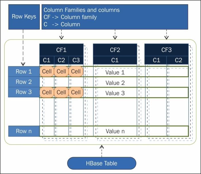
The HBase table is shown in the following figure:
Let's take a look at these components in detail:
· Tables: A Table in HBase is actually more logical than physical. An HBase Table can be described as a collection of rows. The data of a Table is presented in different, multiple Regions, and is distributed by the range of rowkey.
· Rows: A Row is just a logical representation in HBase. Physically, the data is not stored in row, but in columns. Rows in HBase are combinations of columns which can have multiple column families. Each row in HBase is identified by a rowkey which is used as a primary key index. In a Table, rowkey is unique. If a row to be written has an existing rowkey, then the same row gets updated.
· Column Families/Columns: A Column Family is a group of columns which are stored together. Column Families can be used for compression. Designing Column Families is critical for the performance and the utilization of the advantages of HBase. In HBase we store data in denormalization form to create a file which will hold a particular dataset to avoid joins. Ideally, we could have multiple column families in a table but it is not advisable.
One important thing to note is that it is not advisable for a table in HBase to have more than two level Column Family hierarchies, especially if one family has very high data and other has considerably low data. This is because the smaller sized Column Family data will have to be spread across many Regions and flushing and compaction will not be as efficient as a Region impacts adjacent families too.
A Column can be accessed in HBase using the column family and a column qualifier is used to access a column's data, for example, columnfamily:columnname.
· Version/Timestamp: In HBase, a rowkey (row, column, version) holds a cell and we can have the same row and column with a different version to hold multiple cells. HBase stores the versions in descending order of versions so that the recent cell values are found first. Prior to HBase 0.96, the default number of versions kept was three, but in 0.96 and later, it has been changed to one.
· Cell: A cell is where the values are written in HBase. A cell in HBase can be defined by a combination of rowkey {row, column, version} in an HBase Table. The data type will be byte[] and the data stored is called value in HBase.
We can represent the relation of HBase components in the following manner:
(Table, RowKey, ColumnFamily, Column, Timestamp) → Value
ACID properties
HBase does not follow all the attributes of ACID properties. Let's see here how HBase does adhere to specific properties:
· Atomicity: An operation in HBase either completes entirely or not at all for a row, but across nodes it is eventually consistent.
· Durability: An update in HBase will not be lost due to WAL and MemStore.
· Consistency and Isolation HBase is strongly consistent for a single row level but not across levels.
For more details you can check the site http://hbase.apache.org/acid-semantics.html.
The CAP theorem
CAP theorem is also known as Brewer's theorem. CAP stands for:
· Consistency
· Availability
· Partition tolerance
These are the key design properties of any distributed system. We will not get into the details of CAP theorem here but in short, as per the CAP theorem, a distributed system can guarantee only two of the above three properties. As the system is distributed, it has to be Partition tolerant. This leads to two possibilities; either CP, or AP.
HBase has a master-slave architecture. The MasterServer process is single point of failure (we can configure High Availability for the Master which can have a backup Master readily available) while for the RegionServer, recovery from failure is possible but data may be unavailable for some period of time. HBase is actually considered eventually consistent (strongly row level consistent and not strong across levels), and implements consistency and partition tolerance. Hence, HBase is more towards CP than AP.
The Schema design
HBase schema is drastically different from RDBMS schema design as the requirement and the constraints are different. HBase schema should be designed as required by the application and the schema is recommended to be de-normalized. Data distribution depends on the rowkey, which is selected to be uniform across the cluster. Rowkey also has a good impact on the scan performance of the request.
Things to take care of in HBase schema design are as follows:
· Hotspotting: Hotspotting is when one or a few Regions have a huge load of data and the data range is frequently written or accessed causing performance degradation. To prevent hotspotting, we can hash a value of rowkey or a particular column so that the probability of uniform distribution is high and the read and write will be optimized.
· Monotonically increasing Rowkeys/Timeseries data: A problem arising with multiple Regions is that a range of rowkeys could reach the threshold of splitting and can lead to a period of timeout. To avoid this, we should not have the increasing column value as the initial value of rowkey.
· Reverse Timestamp: If we have timestamp in rowkey, the newer data is pushed at the end. If the timestamp is stored like Long.MAX_VALUE timestamp, then the newer data will be present at the start and will be faster and can be avoided, especially in case of a scan.
Let's look at some important concepts for designing schema in HBase:
· Rowkey: Rowkey is an extremely important design parameter in HBase schema as the data is indexed using rowkey. Rowkey is immutable; the only way to change a rowkey is to delete and re-insert it again. Rows are sorted by Rowkeylexicographically, that is, if the rowkey is 1, 32, 001, 225, 060, 45 the order in which the numbers will be sorted would be 001, 060, 1, 225, 32, 45. Table files are distributed across Regions by a range of Rowkey. Usually a combination of sequential and random keys performs better in HBase.
· Column Families: Column Family provides good scalability and flexibility but should be designed carefully. In the current architecture of HBase, no more than two Column Families are advised.
· Denormalize data: As HBase doesn't provide Joins on its own, data should be denormalized. The data will usually be sparse and repeated in many columns, which HBase can take full advantage of.
The Write pipeline
Write pipeline in HBase is carried out by the following steps:
1. Client requests data to be written in HTable, the request comes to a RegionServer.
2. The RegionServer writes the data first in WAL.
3. The RegionServer identifies the Region which will store the data and the data will be saved in MemStore of that Region.
4. MemStore holds the data in memory and does not persist it. When the threshold value reaches in the MemStore, then the data is flushed as a HFile in that region.
The Read pipeline
Read in HBase is performed in the following steps:
1. Client sends a read request. The request is received by the RegionServer which identifies all the Regions where the HFiles are present.
2. First, the MemStore of the Region is queried; if the data is present, then the request is serviced.
3. If the data is not present, the BlockCache is queried to check if it has the data; if yes, the request is serviced.
4. If the data is not present in the BlockCache, then it is pulled from the Region and serviced. Now the data is cached in MemStore and BlockCache..
Compaction
In HBase, the MemStore in Regions creates many HFiles for a Column Family. This large number of files will require more time to read and hence, can impact the read performance. To improve the performance, HBase performs compaction to merge files in order to reduce their number and to keep the data manageable. The compaction process identifies the StoreFiles to merge by running an algorithm which is called compaction policy. There are two types of compactions: minor compactions and major compactions.
The Compaction policy
Compaction policy is the algorithm which can be used to select the StoreFiles for merging. Two policies are possible and the available ones are ExploringCompactionPolicy and RatioBasedCompactionPolicy. To set the policy algorithm, we have to set the value of the property hbase.hstore.defaultengine.compactionpolicy.class of hbase-site.xml. RatioBasedCompactionPolicy was available as the default policy prior to HBase 0.96 and is still available. ExploringCompactionPolicy is the default algorithm from HBase 0.96 and the later version. The difference in these algorithms, in short, is that the RatioBasedCompactionPolicy selects the first set that matches the criteria while the ExploringCompactionPolicy selects the best possible set of StoreFiles with the least work and is better suited for bulk loading of data.
Minor compaction
Minor compaction merges or rewrites adjacent and smaller sized StoreFiles into one StoreFile. Minor compaction will be faster as it creates a new StoreFile and the StoreFiles selected for Compaction are immutable. Please note that Minor compaction does not handle the deleted and expired versions. It occurs when a number of StoreFiles reach a threshold value; to be very specific, the value of the hbase.hstore.compaction.min property in the hbase-site.xml. The default value of the property is 2 and Minor compaction simply merges the smaller file to reduce the number of files. This will be faster as data is already sorted. Some more configurable properties that influence Minor compaction are as follows:
· hbase.store.compaction.ratio: This value determines the balance between the read cost and write cost, a higher value will have a very less number of files having a high read speed and a high write cost. A lesser value will have a lower write cost while the read cost will be comparatively higher. The value recommended is between 1.0 to 1.4.
· hbase.hstore.compaction.min.size: This value indicates the minimum size below which the StoreFiles will be included for compaction. The default value is 128 MB.
· hbase.hstore.compaction.max.size: This value indicates the maximum size above which the StoreFiles will not be included for compaction. The default value is Long.MAX_VALUE.
· hbase.hstore.compaction.min: This value indicates the minimum number of files below which the StoreFiles will be included for compaction. The default value is 2.
· hbase.hstore.compaction.max.size: This value indicates the maximum number of files above which the StoreFiles will not be included for compaction. The default value is 10.
Major compaction
Major compaction consolidates all the StoreFiles of a Region into one StoreFile. The Major Compaction process takes a lot of time as it actually removes the expired versions and deleted data. The initiation of this process can be time triggered, manual, and size triggered. By default, Major Compaction runs every 24 hours but it is recommended to start it manually as it is a write intensive and a resource intensive process, and can block write requests to prevent JVM heap exhaustion. The configurable properties impacting Major Compaction are:
· hbase.hregion.majorcompaction: This denotes the time, in milliseconds, between two Major compactions. We can disable time triggered Major compaction by setting the value of this property to 0. The default value is 604800000 milliseconds (7 days).
· hbase.hregion.majorcompaction.jitter: The actual time of Major Compaction is calculated by this property value and multiplied by the above property hbase.hregion.majorcompaction value. The smaller the value, the more frequent the compaction will start. The default value is 0.5 f.
Splitting
As we discussed about the file and data management in HBase, along with compaction, Splitting Regions also is an important process. The best performance in HBase is achieved when the data is distributed evenly across the Regions and RegionServers which can be achieved by Splitting the Region optimally. When a table is first created with default options, only one Region is allocated to the table as HBase will not have sufficient information to allocate the appropriate number of Regions. We have three types of Splitting triggers which are Pre-Splitting, Auto Splitting, and Forced Splitting.
Pre-Splitting
To aid the splitting of a Region while creating a table, we can use Pre-Splitting to let HBase know initially the number of Regions to allocate to a table. For Pre-Splitting we should know the distribution of the data and if we Pre-Split the Regions and we have a data skew, then the distribution will be non-uniform and can limit the cluster performance. We also have to calculate the split points for the table which can be done using the RegionSplitter utility. RegionSplitter uses pluggable SplitAlgorithm and two pre-defined algorithms available which are HexStringSplit and UniformSplit. HexStringSplit can be used if the row keys have prefix for hexadecimal strings and UniformSplit can be used assuming they are random byte arrays, or we can implement and use our own custom SplitAlgorithm.
The following is an example of using Pre-Splitting:
$ hbase org.apache.hadoop.hbase.util.RegionSplitter pre_splitted_table HexStringSplit -c 10 -f f1
In this command, we use the RegionSplitter with table name pre_splitted_table, with SplitAlgorithm HexStringSplit and 10 number of regions and f1 is the ColumnFamily name. It creates a table called, pre_splitted_table with 10 regions.
Auto Splitting
HBase performs Auto Splitting when a Region size increases above a threshold value, to be very precise, value of property hbase.hregion.max.filesize of hbase-site.xml file which has a default value of 10 GB.
Forced Splitting
In many cases, the data distribution can be non-uniform after the data increases. HBase allows the user to split all Regions of a table or a particular Region by specifying a split key. The command to trigger Forced Splitting is as follows:
split 'tableName'
split 'tableName', 'splitKey'
split 'regionName', 'splitKey'
Commands
To enter in HBase shell mode, use the following:
$ ${HBASE_HOME}/bin/hbase shell
.
.
HBase Shell;
hbase>
You can use help to get a list of all commands.
help
hbase> help
HBASE SHELL COMMANDS:
Create
Used for creating a new table in HBase. For now we will stick to the simplest version which is as follows:
hbase> create 'test', 'cf'
0 row(s) in 1.2200 seconds
List
Use the list command to display the list of tables created, which is as follows:
hbase> list 'test'
TABLE
test
1 row(s) in 0.0350 seconds
=> ["test"]
Put
To put data into your table, use the put command:
hbase> put 'test', 'row1', 'cf:a', 'value1'
0 row(s) in 0.1770 seconds
hbase> put 'test', 'row2', 'cf:b', 'value2'
0 row(s) in 0.0160 seconds
hbase> put 'test', 'row3', 'cf:c', 'value3'
0 row(s) in 0.0260 seconds
Scan
The Scan command is used to scan the table for data. You can limit your scan, but for now, all data is fetched:
hbase> scan 'test'
ROW COLUMN+CELL
row1 column=cf:a, timestamp=1403759475114, value=value1
row2 column=cf:b, timestamp=1403759492807, value=value2
row3 column=cf:c, timestamp=1403759503155, value=value3
3 row(s) in 0.0440 seconds
Get
The Get command will retrieve a single row of data at a time, which is shown in the following command:
hbase> get 'test', 'row1'
COLUMN CELL
cf:a timestamp=1403759475114, value=value1
1 row(s) in 0.0230 seconds
Disable
To make any setting changes in a table, we have to disable a table using the disable command, perform the action, and re-enable it. You can re-enable it using the enable command. The disable command is explained in the following command:
hbase> disable 'test'
0 row(s) in 1.6270 seconds
hbase> enable 'test'
0 row(s) in 0.4500 seconds
Drop
The Drop command drops or deletes a table, which is shown as follows:
hbase> drop 'test'
0 row(s) in 0.2900 seconds
HBase Hive integration
Analysts usually prefer a Hive environment due to the comfort of SQL-like syntax. HBase is well integrated with Hive, using the StorageHandler that Hive interfaces with. The create table syntax in Hive will look like the following:
CREATE EXTERNAL TABLE hbase_table_1(key int, value string)
STORED BY 'org.apache.hadoop.hive.hbase.HBaseStorageHandler'
WITH SERDEPROPERTIES ("hbase.columns.mapping" = ":key,ColumnFamily:Column1, columnFalimy:column2")
TBLPROPERTIES ("hbase.table.name" = "xyz");
Let us understand the syntax and the keywords used for the table:
· EXTERNAL: This is used if the table in HBase exists already, or if the table in HBase is new and you want Hive to manage only the metadata and not the actual data.
· STORED BY: The HBaseStorageHandler has to be used to handle the input and output from HBase.
· SERDEPROPERTIES: Hive column to HBase ColumnFamily:Column mapping has to be specified here. In this example, key maps as a rowkey and value maps to val column of ColumnFamily cf1.
· TBLPROPERTIES: Maps the HBase table name.
Performance tuning
The HBase architecture provides the flexibility of using different optimizations to help the system perform optimally, increase the scalability and efficiency, and provide better performance. HBase is the most popular NoSQL technology due to its flexible Data Model and its interface components.
The components that are very useful and widely used are:
· Compression
· Filters
· Counters
· HBase co-processors
Compression
HBase can utilize compression due to its column-oriented design which is ideal for block compression on Column Families. HBase handles sparse data in an optimal way as no reference or space is occupied for null values. Compressions can be of different types and can be compared depending upon the compression ratio, encoding time, and decoding time. By default, HBase doesn't apply or enable any Compression; for using Compression, the Column Family has to be enabled.
Some compression types which are available to plugin are as follows:
· GZip: It provides a higher compression ratio, but encoding and decoding is slow and space intensive. We can use GZip as compression for infrequent data which needs high compression ratio.
· LZO: It provides faster encoding and decoding, but a lower compression ratio compared to GZip. LZO is under GPL license, hence it's, not shipped along with HBase.
· Snappy: Snappy is the ideal compression type and provides faster encoding or decoding. Its compression ratio lies somewhere between that of LZO and GZip. Snappy is under BSD license by Google.
The code for enabling Compression on a ColumnFamily of an Existing Table using HBase Shell is as follows:
hbase> disable 'test'
hbase> alter 'test', {NAME => 'cf', COMPRESSION => 'GZ'}
hbase> enable 'test'
For creating a new table with compression on a ColumnFamily, the code is as follows:
hbase> create 'test2', { NAME => 'cf2', COMPRESSION => 'SNAPPY' }
Filters
Filters in HBase can be used to filter data according to some condition. They are very useful for reducing the volume of data to be processed, and especially helps save the network bandwidth and the amount of data to process for the client. Filters move the processing logic towards data in the nodes and the result is accumulated and sent to the client. This enhances the performance with a manageable process and code. Filters are powerful enough to be processed for a row, column, Column Family, Qualifier, Value, Timestamp, and so on. Filters are preferred to be used as a Java API, but can also be used from an HBase shell. Filters can be used to perform some ad hoc analysis as well.
Some frequently used filters, like those listed next, are already available and are quite useful:
· Column Value: The most widely used Filter types are Column Value as HBase has a column-oriented architectural design. We will now take a look at some popular Column Value oriented filters:
· SingleColumnValueFilter: A SingleColumnValueFilter filters the data on a column value of an HBase table.
· Syntax:
· SingleColumnValueFilter ('<ColumnFamily>', '<qualifier>', <compare operator>, '<comparator>'
· [, <filterIfColumnMissing_boolean>][, <latest_version_boolean>])
·
· Usage:
· SingleColumnValueFilter ('ColFamilyA', 'Column1', <=, 'abc', true, false)
· SingleColumnValueFilter ('ColFamilyA', 'Column1', <=, 'abc')
· SingleColumnValueExcludeFilter: the SingleColumnValueExcludeFilter is useful to exclude values from a column value of an HBase table.
· Syntax:
· SingleColumnValueExcludeFilter (<ColumnFamily>, <qualifier>, <compare operators>, <comparator> [, <latest_version_boolean>][, <filterIfColumnMissing_boolean>])
· Example:
· SingleColumnValueExcludeFilter ('FamilyA', 'Column1', '<=', 'abc', 'false', 'true')
· SingleColumnValueExcludeFilter ('FamilyA', 'Column1', '<=', 'abc')
· ColumnRangeFilter: The ColumnRangeFilter operates on the Column for filtering the column based on minColumn, maxColumn, or both. We can either enable or disable the minColumnValue constraint by minColumnInclusive_bool Boolean parameter, and maxColumnValue by maxColumnInclusive_bool.
· Syntax:
· ColumnRangeFilter ('<minColumn >', <minColumnInclusive_bool>, '<maxColumn>', <maxColumnInclusive_bool>)
· Example:
· ColumnRangeFilter ('abc', true, 'xyz', false)
· KeyValue: Some filters operate on Key-Value data.
· FamilyFilter: It operates on Column Family and compares each family name with the comparator; it returns all the key-values in that family if the comparison returns true.
· Syntax:
· FamilyFilter (<compareOp>, '<family_comparator>')
· QualifierFilter: It operates on the qualifier and compares each qualifier name with the comparator.
· Syntax:
· QualifierFilter (<compareOp>, '<qualifier_comparator>')
· RowKey: Filters can also work on row level comparison and filter data.
· RowFilter: Compares each row key with the comparator using the compare operator.
· Syntax:
· RowFilter (<compareOp>, '<row_comparator>')
· Example:
· RowFilter (<=, 'binary:xyz)
· Multiple Filters: We can add a combination of Filters to a FilterList and scan them. We can choose to have OR, or AND between the filters by using:
· FilterList.Operator.MUST_PASS_ALL or FilterList.Operator.MUST_PASS_ONE.
· FilterList list = new FilterList(FilterList.Operator.MUST_PASS_ONE);
· // Use some filter and add it in the list.
· list.add(filter1);
· scan.setFilter(list);
We have many other useful filters which are available and if we need, then we can also create a custom based filter.
Counters
Another useful feature of HBase is Counters. They can be used as a distributed Counter to increment a column value, without the overhead of locking the complete row and reducing the synchronization on Write, for incrementing a value. Incrementing or counters are required in many scenarios, especially in many analytical systems like digital marketing, click stream analysis, document index models, and so on. HBase Counters can manage with very less overhead. Distributed Counter is very useful but poses different challenges in a distributed environment as the counter values will be present in multiple servers at the same time and the write and read requests will be considerably high. Therefore, to be efficient, we have two types of Counters present in HBase which are single and multiple counters. Multiple counters can be designed to count in an individual hierarchical level according to rowkey distribution and can be used by summing up the Counters to get the whole counter value. The types of counter are explained as follows:
· Single Counter: Single Counters work on specified columns in the HTable, row wise. The methods for Single Counters provided for an HTable, are as follows:
· long incrementColumnValue(byte[] row, byte[] family, byte[] qualifier,long amount) throws IOException
long incrementColumnValue(byte[] row, byte[] family, byte[] qualifier,long amount, boolean writeToWAL) throws IOException
We should use the second method with writeToWAL to specify whether the write-ahead log should be active or not.
· Multiple Counter: Multiple Counters will work qualifier-wise in the HTable. The method for Multiple Counters provided for an HTable is as follows:
Increment addColumn(byte[] family, byte[] qualifier, long amount)
HBase coprocessors
Coprocessor is a framework which HBase provides to empower and execute some custom code on RegionServers. Coprocessors move the computation much closer to the data, specifically Region-wise. Coprocessors are quite useful for calculating aggregators, secondary indexing, complex filtering, auditing, and authorization.
HBase has some useful coprocessors implemented and open for the extension and custom implementation of a Coprocessor. Coprocessors can be designed based on two strategies- Observer and Endpoint, which are as follows:
· Observer: As the name suggests, Observer coprocessors can be designed to work as a callback or in case of some event. Observers can be thought of as triggers in RDBMS and can be operated at Region, Master, or WAL levels. Observers have the PreXXX and PostXXX conventions for methods to override, before and after an event respectively. The following are the types of Observer according to the different levels:
o RegionObserver: The Region Observers process Region level data. These can be used for creating secondary indexes to aid retrieval. For every HTable Region, we can have a RegionObserver. RegionObserver provides hooks for data manipulation events, such as Get, Put, Delete, Scan, and so on. Common example include preGet and postGet for Get operation and prePut and postPut for Put operation.
o MasterObserver: The MasterObserver operates at the Master Level where the DDL-type operations like create, delete, and modify table are processed. Extreme care should be taken to utilize MasterObserver.
o WALObserver: This provides hooks around the WAL processing. It has only two methods; preWALWrite() and postWALWrite().
· Endpoint: Endpoints are operations which can be called via a client interface by directly invoking it. If Observers can be thought of as triggers, then Endpoint can be thought of as Stored Procedures of RDBMS. HBase can have tens of millions of rows or many more; if we need to compute an aggregate function, like a sum on that HTable, we can write an Endpoint coprocessor which will be executed within the Regions and will return the computed result from a Region as in map side processing. Later from all Regions result can perform the sum as in reduce side processing. The advantage of Endpoint is that the processing will be closer to the data and the integration will be much more efficient.
Summary
In this chapter, you have learned that HBase is a NoSQL, Column-oriented database with flexible schema. It has the following components – MasterServer, RegionServer, and Regions and utilizes Zookeeper to monitor them with two caches – WAL in RegionServers and MemStore in Regions. We also saw how HBase manages the data by performing RegionSplitting and Compaction. HBase provides partition tolerance and much higher consistency levels as compared to availability from the CAP theorem.
The HBase Data Model is different from the traditional RDBMS as data is stored in a column oriented database and in a multidimensional map of key-value pairs. Rows are identified by rowkey and are distributed across clusters using a range of values of rowkey. Rowkey is critical in designing schema for HBase for performance and data management.
In a Hadoop project, data management is a very critical step. In the context of Big Data, Hadoop has the benefit of the data management aspect. But managing it with some scripts becomes difficult and poses many challenges. We will cover these in the next chapter with tools that can help us in managing the data with Sqoop and Flume.
All materials on the site are licensed Creative Commons Attribution-Sharealike 3.0 Unported CC BY-SA 3.0 & GNU Free Documentation License (GFDL)
If you are the copyright holder of any material contained on our site and intend to remove it, please contact our site administrator for approval.
© 2016-2026 All site design rights belong to S.Y.A.