Using JMP 12 (2015)

Chapter 3. Import Your Data

Create Data Tables

This chapter covers the following topics:

•How to import data into JMP, such as text files, SPSS files, and SAS data

•How to transfer Excel data into a JMP data table

•How to read in real-time data

•How to create a new data table

Figure 3.1 Importing a Text File

Contents

About Importing Data to JMP

Import Microsoft Excel Files

Import Data from SAS

Import SAS Data Sets

Create SAS Transport Files in SAS

Connect to SAS

Open SAS Data Sets with SAS Query Builder

Open SAS Data Sets through a SAS Server

Run Stored Processes

Submit SAS Code

Generate ODS Results

Retrieve Generated SAS Data Sets

Build SQL Queries in Query Builder

Import Data from a Database

Import Text Files

Import Remote Files and Web Pages

Import SPSS Files

Import Data from R

Import Data Using the Excel Add-In

Create New Data Tables

About Importing Data to JMP

You can import many file formats into JMP and save them as data tables. JMP opens many files by default. The file formats which JMP does not support by default require specific Open Database Connectivity (ODBC) drivers.

The Following File Formats Are Supported by Default:

•Comma-separated (.csv)

•.dat files that consist of text

•ESRI shapefiles (.shp)

•Flow Cytometry versions 2.0 and 3.0 (.fcs)

•HTML (.htm, .html)

•MATLAB (.m, .M)

•Microsoft Excel 1997 through 2011 (.xls, .xlsx on Macintosh)

•Microsoft Excel 2007 through 2013 (*.xlsx, *.xlsm on Windows)

•Minitab Portable Worksheet (.mtp)

•Plain text (.txt)

•R (.r)

•SAS transport (.xpt, .stx)

•SAS versions 7 through 9 on Macintosh (.sas7bdat)

•SAS versions 7 through 9 on Windows (.sas7bdat, .sas7bxat)

•SPSS files (.sav)

•Tab-separated (.tsv)

•Teradata database (.trd)

•xBase data files (.dbf)

Notes on SAS Support:

On both Windows and Macintosh, you can open SAS data sets directly through the File > Open command. Another option is connecting to a SAS server by selecting File > SAS > Browse Data. See “Import SAS Data Sets” for details about opening SAS data sets directly. See “Open SAS Data Sets through a SAS Server” for details about connecting through a SAS server.

The Following Files Require ODBC Drivers:

•Database (dBASE) (.dbf, .ndx, .mdx) is supported with a V3+ compliant ODBC driver.

•Microsoft Access Database (.mdb) is supported with a V3+ compliant ODBC driver.

See “Import Data from a Database” for details for working with databases.

Your computer’s available memory affects data import. Very large files might load slowly or not at all. Consider splitting up large files before importing them. In JMP, you can then join or concatenate the tables. For more information, see “Concatenate Data Tables” in the “Reshape Data” chapter and “Join Data Tables” in the “Reshape Data” chapter.

Note: You can open R code (.R) and SAS program files (.sas) in JMP, but the text opens in a Script window, not in a data table.

Import Microsoft Excel Files

Microsoft Excel files are converted to data tables in JMP. The first row becomes column headers, data in merged cells can be displayed in separate cells, and other worksheet features are preserved.

Microsoft Excel files open in the Excel Import Wizard by default. JMP detects how the data is structured and provides a preview of the data table. You can then modify the settings before importing the data. For example, indicate which row the data begin on and whether the worksheet contains column headers or hidden rows or columns. Microsoft Excel .xls, .xlsm, and .xlsx file formats are supported.

For information about opening a Microsoft Excel file outside the wizard, see “Import a Microsoft Excel File Directly”.

Notes:

•Password-protected Microsoft Excel .xlsx files cannot be opened in JMP.

•Between Windows and Macintosh, the number of digits after a decimal point and the date format of imported data might differ. For example, “10/25/2012” might be formatted as “25Oct2012” on Macintosh. Columns might be imported as character columns on Macintosh but not on Windows.

Preview and Import the Microsoft Excel Data

Before you import a worksheet, it is helpful to know whether the worksheet includes hidden or merged cells. In the wizard, you can then exclude hidden columns or rows. Another option is to duplicate the data that were previously merged in the worksheet.

To import a Microsoft Excel file that contains several worksheets, follow these steps:

1.Open the file in Microsoft Excel.

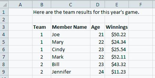
For the figures in this example, we used the Team Results.xlsx file located in the JMP Samples/Import Data folder. The file has the following characteristics:

‒the data begin on row 4, column 2 and end on row 9, column 5

‒two worksheets

‒the second worksheet has two sets of merged cells

‒no hidden rows or columns

Figure 3.2 Team Results.xlsx Worksheet

2.To open an Excel file in JMP, selectFile > Open.

The Open Data File window appears.

3.Select the Excel file.

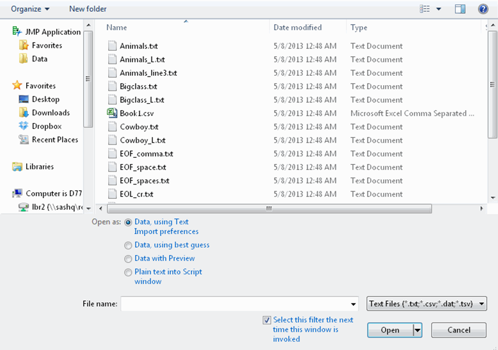
Figure 3.3 Open Data File Window

•The Open window includes an option to Select this filter the next time this window is invoked. Select to enable this option if you plan to open .xlsx files every time.

•The Open window also includes an option to configure Excel file imports to Always enforce Excel Row 1 as labels. Select to have JMP Always use row 1 of the Excel file as column labels, Never use row 1 as labels, or allow JMP to use Best Guess.

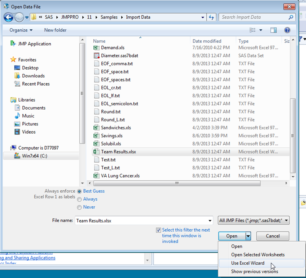
4.Click theOpendown arrow to show the menu.

‒To only open selected worksheets, select Open Selected Worksheets.

A window appears that allows you to select a subset of worksheets to import.

Or

‒Select Use Excel Wizard to use JMP’s Excel Wizard to import the worksheet.

The worksheet opens in the Excel Import Wizard, where a preview of the data appears along with import options (Figure 3.4).

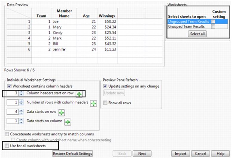
Figure 3.4 Example Initial Data Preview

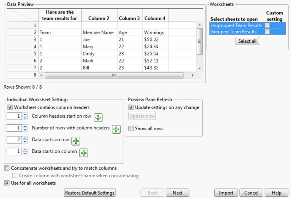
Note the following characteristics in the Data Preview:

‒Both worksheets are selected for import.

‒The first column has been automatically been removed.

‒Text from the first row of the worksheet appears as the column headings. However, you want the text in row 3 of the worksheet to be used as the column headings.

‒The first data row is empty.

Note: JMP can remember your previous changes each time you import a worksheet, even after closing and reopening JMP. This feature is helpful when you want to reimport the same worksheet several times and experiment with options. To clear those changes when you import a different worksheet, click Restore Default Settings.

5.To have the Data Preview automatically refresh when you make changes, selectUpdate settings on any change.

However, if the file is very large, automatically refreshing the Data Preview could take a lot of time. Deselect Update settings on any change. Then after making your changes, click Update now to manually refresh the Data Preview.

6.In the Worksheets pane (upper right corner), select the worksheet to import (for example, Ungrouped Team Results) (Figure 3.5). SelectSelect Allto highlight the entire list of worksheets.

Note: If you plan to concatenate two or more worksheets, select the worksheets in the Worksheets pane. You must select at least two worksheets for table concatenation to work.

7.If the worksheet contains rows with column headers, selectWorksheet contains column headers.

Or

If the worksheet does not contain rows that are column headers, deselect this option to disable column header configuration settings.

8.If the worksheet has a row with column headers, click the up arrow of theColumn headers start on rowspin buttonuntil the header row appears correct (for this example, click the up arrow twice) (Figure 3.5).

Or

Type the row number in the Column headers start on row text box (for example, 3) and press ENTER.

Note: The value for Data starts on row was changed from 2 to 4 (Figure 3.5).

9.If the worksheet has multiple rows as column headers, click the up arrow of theNumber of rows with column headersspin buttonuntil the header rows appear correctly.

Or

Type the number of rows in the Number of rows with column headers text box and press ENTER.

10.If the data start on a different row from the row displayed in the Data Preview, use the spin button or type the row number in theData starts on row.

11.If the data start on a different column number from the column displayed in the Data Preview, use the spin button or type the column number in theData starts on column.

12.To have all worksheets in the file merged into one data table and have JMP try to match columns, selectConcatenate worksheets and try to match columns.

‒If worksheets are concatenated, select Create column with worksheet name when concatenating to have JMP add a new Source Table column that lists the worksheet name for each imported table.

13.To save the settings only for this worksheet, deselectUse for all worksheetsin the lower left corner of the window.

Or

To use the same settings for all worksheets in the file, select Use for all worksheets.

Figure 3.5 Selecting the Column Header Row

14.ClickNextto configure other import settings.

The window displays additional import configuration settings.

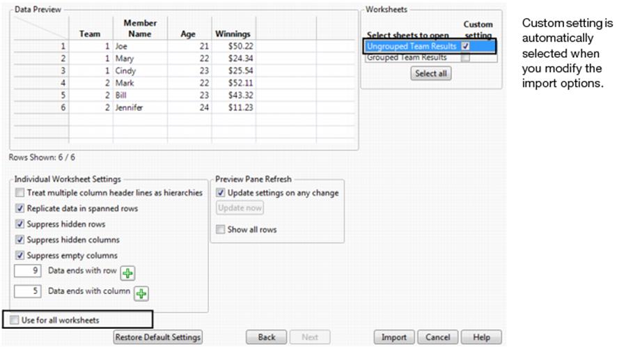
15.If the worksheet contains multiple rows as column headers and you want these to be hierarchies, selectTreat multiple column header lines as hierarchies.

16.If the worksheet contains merged cells across rows, selectReplicate data in spanned rowsto have JMP unspan the cells and copy the cell contents into all of the resulting cells.

If you deselect Replicate data in spanned rows, JMP unspans the cells and copies the cell contents into the topmost cell. The remaining unspanned cells are left empty.

Note: JMP automatically unspans cells that span columns and copies the cell contents into all of the resulting cells.

17.To disregard any hidden rows during the import, selectSuppress hidden rows.

18.To disregard any hidden columns during the import, selectSuppress hidden columns.

19.To import an empty column that has a column header, deselectSuppress empty columns.

By default, empty columns are not imported.

20.To restrict the number of rows to import, type the last row number in theData ends with rowtext box (for example, 9).

21.To restrict the number of columns to import, type the last column number in theData ends with columntext box (for example, 5).

The data preview is updated as shown in Figure 3.6.

Figure 3.6 Specifying the Last Column

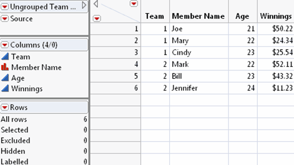
22.ClickImportto convert the worksheet as you specified (Figure 3.7).

Figure 3.7 Final Data Table

Tips:

•JMP can remember your previous changes each time you import a worksheet, even after closing and reopening JMP. This feature is very helpful when you want to reimport the same worksheet several times and experiment with options. To clear those changes when you import a different worksheet, click Restore Default Settings.

•Your import settings are saved in a data table script named Source. To reimport the worksheet using the same settings, run the script. The script includes the path to the worksheet, so make sure that other users have access to that location if necessary.

•As you experiment with settings for a large worksheet, the data preview might be slightly delayed. To speed up the preview, deselect Update settings on any change on the first wizard window. Modify the settings and then click Update now to refresh the data preview.

•To view all rows in the Data Preview pane, select Show all rows. The preview might be slightly delayed depending on the size of the spreadsheet.

•You can combine two worksheets from the same workbook into one data table. The column names are matched on import, so the order of the columns is irrelevant.

Import a Microsoft Excel File Directly

Microsoft Excel files open in the Excel Import Wizard by default. This option is helpful when the structure of data in the worksheet is irregular. For example, you might want to exclude hidden columns or convert text in the third row to column headings.

You can also select File > Open to open a Microsoft Excel file. For example, JMP can convert the first row to column headings.

JMP also opens Excel files from web sites that do not require you to log on. On Windows, follow the procedure in this section. On Macintosh, use the File > Internet Open command. See “Import Remote Files and Web Pages” for more information.

To set the Excel Open Method preference

To always open Microsoft Excel files directly, change the Excel Open Method preference. Choose to open all worksheets at once or select them from a list. The Excel Open Method preference is in File > Preferences > General (Windows) and JMP > Preferences > General(Macintosh).

To open a Microsoft Excel file (Windows)

1.Select File > Open.

2.Select theExcel Filesfile type, select the file, or enter the URL.

3.(Optional) To convert text in the first row to column headings, selectAlwaysnext toAlways enforce Excel Row 1 as labels.If you do not want to import specific worksheets, clickOpen.

4.(Optional) Click theOpenbutton arrow, and then selectOpen Selected Worksheets.

A window appears that allows you to select a subset of worksheets to import.

‒Select one or more worksheets and click OK.

To open a Microsoft Excel file (Macintosh)

1.Select File > Open and select the file.

2.(.xlsonly) To convert text in the first row to column headings, selectUse Excel Labels as Headings.

3.(.xlsonly) To open specific worksheets, selectSelect Individual Excel Worksheets.

4.ClickOpen.

If you chose to open specific worksheets, select those worksheets from the list, and then click OK. You can also click Select All if you change your mind and want to import all worksheets.

Import Data from SAS

You can connect to a SAS server and work directly with SAS data sets:

•Import whole SAS data sets or portions of data sets

•Make changes to imported SAS data in JMP and then export those changes as a SAS data set

•Run stored processes

•Submit SAS code from JMP

Java Runtime Environment (JRE) Requirements

•On Windows, Java Runtime Environment (JRE) 7 or later must be installed on your computer to access SAS. However, JRE 7 does not need to be specified as the current version.

•On Macintosh, JRE 7 or later must be installed for SAS integration.

Access SAS options from the File > SAS menu:

Browse Data

Browse and import data residing on a SAS Server.

SAS Query Builder

Select and import data from an SQL database on a SAS server without writing SQL statements. See “Build SQL Queries in Query Builder” for details.

Export Data to SAS

Export JMP data tables to a SAS Server.

Browse SAS Folders

Browse and run SAS stored processes or open Metadata-defined data tables.

New SAS Program

Opens a script window for writing and submitting SAS code.

Submit to SAS

Sends SAS code directly from JMP to the currently active SAS server.

Open SAS Log Window

Opens a SAS log window for the active SAS server.

Open SAS Output Window

Opens a SAS output window for the active SAS server. This window shows recent SAS output.

Server Connections

Administer connections to SAS servers.

You can also find shortcuts for SAS options on the SAS page of the JMP Starter, and there is a SAS toolbar. You can save certain settings pertaining to SAS Integration on the SAS Integration page of the Preferences window (File > Preferences). For more information about setting your SAS Integration preferences, see “SAS Integration” in the “JMP Preferences” chapter.

Import SAS Data Sets

SAS data sets are saved in one of many SAS formats:

•Windows supported formats are .sas7bdat and .sas7bxat.

•Macintosh supports reading and writing .sas7bdat files.

•Windows and Macintosh support reading and writing .xpt files

When you open a data set in JMP, the file opens as a data table. JMP uses SAS variable names as column names by default. To use variable labels in a specific file on Windows, select the option when you open the file (see step 5 below).

To open a SAS data set:

Note: On Macintosh, select File > Open, select the data set, and then click OK.

1.Select File > Open.

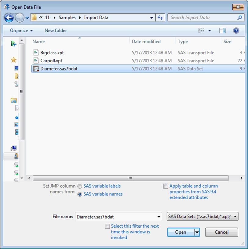
2.(Windows only) SelectSAS Data Setsfrom the list next toFile nameas shown inFigure 3.8.

Note: SAS variable names and formats are preserved and can be saved after changes are made to the SAS data set. See “Save as a SAS Data Set” in the “Save and Share Data” chapter.

3.Select the file.

Figure 3.8 Open SAS Data Set

4.(Optional) Select any of the following options:

‒SAS variable labels  Uses the SAS variable labels (instead of variable names) as the column names in the JMP data table.

‒SAS variable names  Uses the SAS variable names (instead of the labels) as the column names in the JMP data table.

5.(Optional on Windows) Select any of the following options:

‒Apply table and column properties from SAS 9.4 extended attributes  If the SAS server supports extended attributes (SAS 9.4), includes the extended attributes when storing JMP metadata. This setting overrides the SAS 9.4 Extended Attributes preference on the SAS Integration page.

‒Select this filter the next time this dialog is invoked Sets the default file type choice to the option that you select next to the File name list If selected, the default file type will be SAS Data Sets the next time you reach this window.

6.(Optional) Select any of the following for a SAS Transport (.xpt) file:

‒Select member Lets you enter the name of a specific member, or table, for JMP to open. On Macintosh, select Member Tables > Specified and then enter the name.

‒Open all members Opens all members, or tables, in the transport file. On Macintosh, select Member Tables > All.

‒Save all members Saves the file as a JMP file as soon as you open it. The file is saved to the same directory where the SAS transport file was opened. On Macintosh, the option is Save all.

‒Select Columns Tells JMP to open only certain columns from the transport file. Select the columns that you want to import from the list that appears. On Macintosh, the option is Select columns before opening.

7.ClickOpen.

Note: If you are importing date variables from a SAS file, JMP looks for a SAS date format and translates it to a JMP date column.

Create SAS Transport Files in SAS

JMP can open SAS transport files that were saved using the SAS XPORT engine. For example, below is sample SAS code that creates a transport file called test.

Note: misc and work are SAS libref names.

data test;

input name $ age weight;

cards;

Susan 12 72

Melanie 10 68

Jonathan 11 77

Sheila 13 67

;

libname misc xport 'C:/test.xpt';

proc copy in=work out=misc;

run;

Connect to SAS

You can either connect to a SAS Metadata Server or directly to a SAS Workspace Server. Once connected to a SAS Metadata Server, you can browse through SAS servers, libraries, and data sets.

Note: SAS Server version 9.4 is the default setting in the JMP SAS Integration preferences. The earliest supported release of the SAS Metadata Server is version 9.1.3 SP4. Connections to earlier releases of the SAS Metadata Server are experimental and are not supported.

To begin, select File > SAS > Server Connections. The SAS Server Connections window shown in Figure 3.9 appears. All connections are made in this window.

Figure 3.9 SAS Server Connections

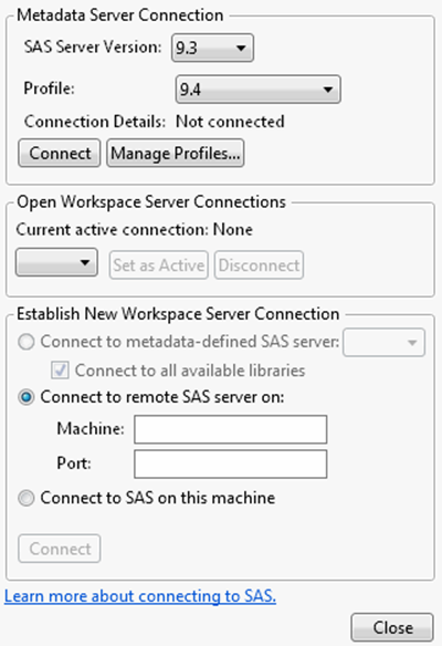
The following sections describe how to connect to a SAS server.

•“Connect to a SAS Metadata Server”

•“Connect to a Remote SAS Workspace Server”

•“Connect to a SAS Environment (Windows Only)”

•“Connect to SAS on Your Local Machine (Windows Only)”

Connect to a SAS Metadata Server

Note: You can be connected to only one Metadata Server at a time. If you make a second connection, your first one is disconnected.

To connect to a Metadata Server

1.Select File > SAS > Server Connections. The SAS Server Connections window shown in Figure 3.9 appears.

2.Select the version for the SAS Server. Your SAS Metadata Server administrator should have this information.

SAS Server version 9.4 is selected by default based on the JMP SAS Integration preferences.

3.Select the profile that you want to use.

If you do not have a profile set up, see “To create or modify a SAS Metadata Server profile”.

4.ClickConnect.

If JMP is unable to establish a connection, an error message appears. Common reasons are invalid user names or passwords. If you need to update the information for the profile, see “To create or modify a SAS Metadata Server profile”.

5.ClickClose.

Once you are connected to a SAS Metadata Server, you can connect to any SAS Workspace Servers that the Metadata Server offers.

To connect to a SAS Workspace Server (Windows only)

1.Select File > SAS > Server Connections. The SAS Server Connections window shown in Figure 3.9 appears.

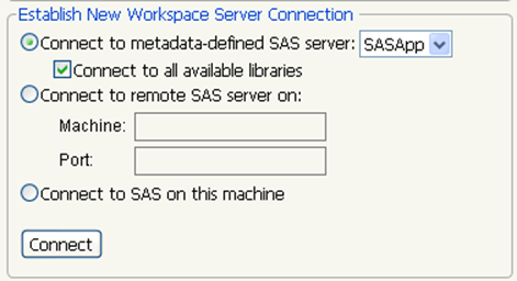
2.Select the Workspace Server to connect to (Figure 3.10).

Figure 3.10 Open a Connection to a Workspace Server

3.ClickConnect.

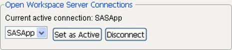
Under Open Workspace Server Connections, the Workspace Server is shown as the current active connection. See Figure 3.11.

Figure 3.11 Current Active Connection

4.ClickClose.

To change the active connection

Note: The active connection is what is used to submit SAS code or handle SAS script commands.

To change the active connection, you first need to be connected to more than one server. Follow the instructions in “To connect to a SAS Workspace Server (Windows only)” to add two or more server connections.

1.In the Open Workspace Server Connections section, click the drop-down menu and select the desired server.

2.ClickSet as Active.

3.ClickClose.

Tip: You can change the active server at any time.

To disconnect from a SAS Workspace Server

1.In the SAS Server Connections window, select the Workspace Server to disconnect under Open Workspace Server Connections.

2.ClickDisconnect.

To disconnect from a SAS Metadata Server

1.In the SAS Server Connections window, select the Metadata Server to disconnect.

2.ClickDisconnect.

To create or modify a SAS Metadata Server profile

1.In the SAS Server Connections window, select the SAS Server Version.

2.ClickManage Profiles.

3.ClickAddto add a new profile, or clickModifyto change a profile’s settings.

The Create Profile or Modify Profile window appears. If you are adding a new profile, all fields are empty except the Authentication domain field, which contains DefaultAuth, and the Port field. If you are modifying a profile, the fields contain the current information.

Figure 3.12 Create or Modify a Metadata Server Profile

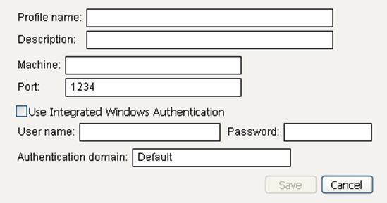
4.Fill in the information needed to connect to a SAS Metadata Server. Your SAS Metadata Server administrator should have this information.

Profile name

Select a name for this profile. This name is shown in the list of profiles.

Description

(Optional) You can enter a short description of this profile.

Machine

The name of the machine that hosts the Metadata Server. (Example: myserver.mycompany.com)

Port

The port through which you should connect to the machine. (Example: 8561)

Use Integrated Windows Authentication

Select this option to use your Windows log in ID and password to access the server. When enabled, the User name and password fields are disabled. This option is disabled by default.

User name

Your user name for the Metadata Server.

Password

Your password. This is always displayed as asterisks.

Authentication domain

The domain you, as a user, belong to.

5.ClickSave.

Connect to a Remote SAS Workspace Server

You can also connect directly to a SAS Workspace Server, instead of going through a Metadata Server.

To connect to a Remote SAS Workspace Server

1.Select File > SAS > Server Connections. The SAS Server Connections window shown in Figure 3.9 appears.

2.Under Establish New Workspace Server Connection, selectConnect to remote SAS server on. SeeFigure 3.13.

Figure 3.13 Open a Connection to a Remote SAS Server

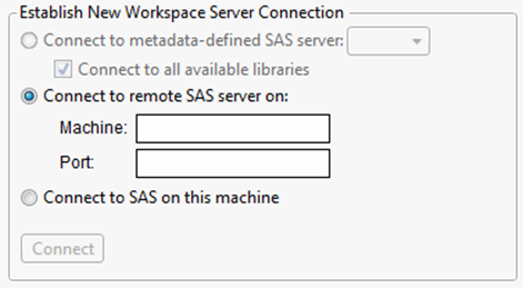
3.Enter the machine name and the port number. Your SAS server administrator has this information.

4.ClickConnect.

5.Enter your user name and password in the window that appears.

6.ClickOK.

7.ClickClosein the SAS Server Connections window.

To disconnect from a Remote SAS Workspace Server

1.In the SAS Server Connections window, select the server to disconnect under Open Workspace Server Connections.

2.ClickDisconnect.

Connect to a SAS Environment (Windows Only)

On Windows, you can connect to a SAS mid-tier (or SAS environment) if SAS Server version 9.3 or 9.4 is selected in JMP’s preferences and your computer or JMP has been configured correctly. (SAS Server version 9.4 is the default setting in the JMP SAS Integration preferences.)

The SAS installer should have set up your computer to find the SAS environment definition file. If not, you can enter the path to the file in the JMP preferences.

To configure your JMP preferences

1.Select File > Preferences > SAS Integration.

2.SelectI want to connect to a SAS Environmentand then clickConfigure.

3.To connect to an environment that JMP has already detected, clickAutomatic discovery,and then select the URL from the list if necessary.

4.To enter the path to the SAS environment definition file, clickManual configurationand enter the URL.

5.ClickOK.

To connect to a SAS Environment

1.Select File > SAS > Server Connections to open the SAS Server Connections window.

2.In the Metadata Server Connection area, selectConnect to a SAS Environment.

If this option is not available, either your computer or JMP is not configured to find the environment. See “To configure your JMP preferences” for details.

3.Select the name of the environment from the Environment list if necessary.

4.ClickConnect.

5.Enter your user name and password if prompted.

Connect to SAS on Your Local Machine (Windows Only)

You can also connect directly to SAS on your local machine.

To connect to SAS on your computer

1.Select File > SAS > Server Connections to open the SAS Server Connections window.

2.Under Establish New Connection, selectConnect to SAS on this machine.

This option is disabled if SAS is not installed on the computer.

3.ClickConnect.

4.ClickClosein the SAS Server Connections window.

To disconnect from SAS on your computer

1.In the SAS Server Connections window, select Local under Open Connections.

2.ClickDisconnect.

Open SAS Data Sets with SAS Query Builder

SAS Query Builder is the preferred method for selecting and importing data from an SQL database on a SAS server. You can preview the data before importing it into a data table. You can also save the queries to modify and run later or to reference in a JSL script.

SAS Query Builder provides an alternative to opening SAS data sets with the File > SAS > Browse Data feature.

To open a SAS data set with SAS Query Builder, follow these steps:

1.Select File > SAS > SAS Query Builder.

2.In the Connect to SAS Server window, select a Metadata server or a remote server.

‒To connect to a Metadata server that you have already set up in JMP, select the server from the Connect to metadata-defined SAS server list.

‒To add or configure a Metadata server, click Manage Profiles and follow steps in “To create or modify a SAS Metadata Server profile”.

‒To connect to a remote server, enter the machine name and the port number. Your SAS Metadata Server administrator should have this information.

3.ClickOK.

The SAS Query Builder window appears.

For details about using Query Builder, see “Build SQL Queries in Query Builder”.

Notes:

•All Query Builder queries run in the foreground.

•Extended attributes are not imported by default. To import them, modify the JMP SAS Integration preferences. Select File > Preferences (Windows) or JMP > Preferences (Macintosh). Select SAS Integration and then select On import, apply table and column properties from extended attributes.

•SAS Query Builder does not support local server connections.

Open SAS Data Sets through a SAS Server

Once you connect to a SAS Workspace Server, you can browse through the SAS libraries on that server and import data into JMP.

To browse the data sets on the SAS server, select File > SAS > Browse Data. The Browse SAS Data window appears. See Figure 3.14.

Figure 3.14 Browse SAS Data

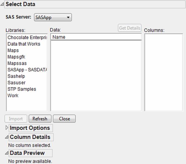
The window is initially populated with a list of servers the SAS Metadata Server provides (if connected). Any physical and local connections are also shown (as listed in Figure 3.13).

•Select a server to see a list of libraries that server contains.

•Select a library to see a list of data sets within that library.

•Select a data set to see a list of columns within that data set.

When you close and reopen the Browse SAS Data window, the previously viewed library and data set appear in the window. However, at any time, you can select a different server from the SAS Server list and then select a library and data set.

Tip: If a server is unavailable, or if the connections failed, the server’s name is shown in light, italic text. Click it to try to re-establish the connection.

Browse SAS Data Information

You can select a SAS data set and see information about its contents before opening it using the Get Details, Column Details, and Data Preview options.

Data Preview

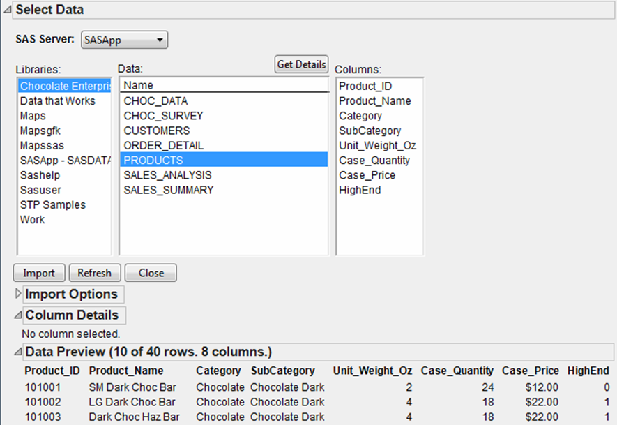
When you select a data set, the Data Preview outline shows you the first ten rows and columns in the data set. See Figure 3.15.

Figure 3.15 Data Preview

Data Set Details

Click Get Details in the Browse SAS Data window to see the size and last modification date for each data set in the library. This option helps you estimate whether your computer can process the entire data set.

Column Details

To see information about a particular column in the data set, select it. The Column Details outline shows you some basic information about the data column. See Figure 3.16.

Figure 3.16 Column Details

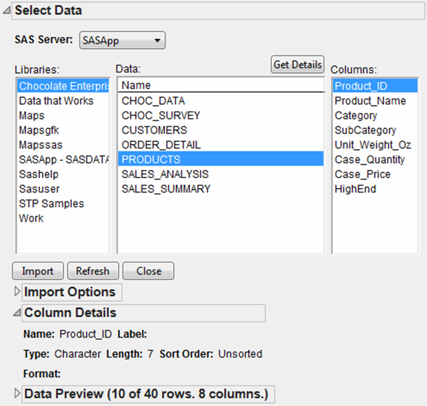
Name

Column name from the SAS data set.

Label

Descriptive column label. The label can be longer than the name, and is often helpful to determine what the column name means.

Type

Specifies whether the column has a character or numeric data type.

Length

The length in bytes of data in the column.

Sort Order

How the column is sorted in SAS.

Format

The format for the SAS column, such as DOLLAR. This format field also contains information about the width of formatted values and the number of decimal places.

Open a SAS Data Set in JMP

You can import SAS data sets directly into JMP.

1.From the Browse SAS Data window, select a data set.

By default, JMP specifies All rows for import.

2.ClickImport.

The entire SAS data set is imported into a JMP data table. When SAS data is imported, JMP attempts to make the best match to the SAS format.

Import a Sample of a SAS Data Set

You can import a sample of a SAS data set directly into JMP.

1.From the Browse SAS Data window, select a data set.

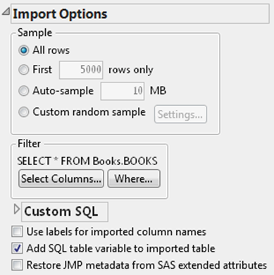
2.Open the Import Options outline. SeeFigure 3.17.

Figure 3.17 Import Options

3.If you want to import only a portion of a data set, you can do any of the following:

‒Select the first x number of rows only. See “To import the first x number of rows only”.

‒Select to auto-sample a specified file size. See “To import an auto-sample file of a specified size”.

‒Select a subset of the columns. See “To select a subset of columns”.

‒Construct a WHERE clause to filter the data. See “To import using a WHERE clause”.

‒Take a custom sample of the data. See “Importing a Random Sample of the Data”.

To import the first x number of rows only

1.In the Import Options section, select First x rows only and specify the number of rows to import.

2.In the Browse SAS Data window, clickImport.

JMP imports the specified number of rows.

To import an auto-sample file of a specified size

1.In the Import Options section, select Auto-sample and specify the number of MB to import.

2.In the Browse SAS Data window, clickImport.

JMP imports the specified number of MB.

To select a subset of columns

1.In the Import Options section, click Select Columns.

The Select Columns window appears. See Figure 3.18.

Figure 3.18 Select Columns

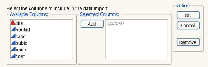
2.Select the columns that you want to import.

To select more than one column at a time, press CTRL and click each column.

3.ClickAdd.

4.When you have added all the columns that you want, clickOK.

5.In the Browse SAS Data window, clickImport.

Only the columns that you selected from the SAS data set are imported into a JMP data table.

To import using a WHERE clause

1.Click Where.

2.Use the WHERE clause editor to construct your WHERE clause.

3.ClickOKto return to the Browse SAS Data window.

4.ClickImport.

Only the data that matches your WHERE clause are imported into a JMP data table.

For information about constructing WHERE clauses and using the WHERE clause editor, see “Use the WHERE Clause Editor”.

Note: If you import data using both a WHERE clause and sampling, the WHERE clause is applied first, and then a sample of the filtered data is taken.

You can also write your own SQL statements.

To import using a custom SQL statement

You can also open a SAS data set using a custom SQL statement.

1.Open the Custom SQL outline under the Import Options outline. See Figure 3.17.

Figure 3.19 Custom SQL

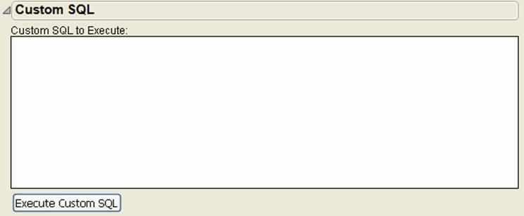
2.Enter your SQL statement in the window.

3.ClickExecute Custom SQL.

Note: Your SQL is run on the selected server but is not restricted to any selected library or data set.

Importing a Random Sample of the Data

You can also import a random sample of the rows of the SAS data set.

Note: The sampling feature requires that the SAS server has the SAS/STAT product licensed and installed. If SAS/STAT is not present, sampling is disabled.

In the Sample Imported Data area of the Import Options outline, select the Custom random sample check box. By default, 5% of the rows are imported. To change the random sample import settings, click the Settings button.

Figure 3.20 Sampling Settings

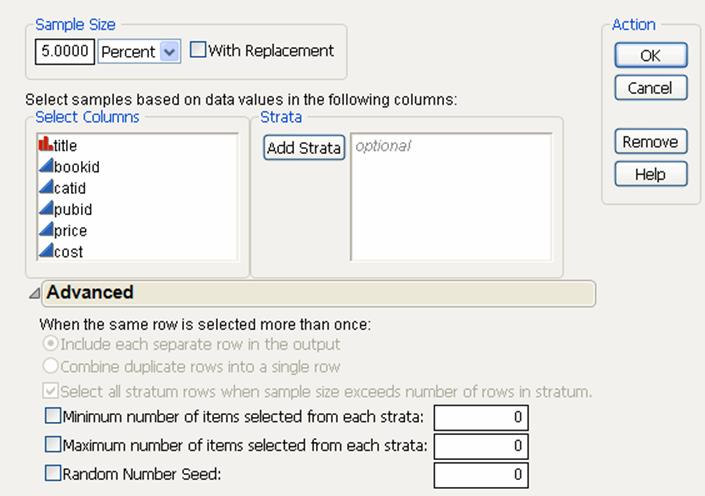
In this window, you specify any of the following:

Sample Size

You can set the sample size be percentage or by number of rows. To ensure that each row is sampled only once, de-select the With replacement option. To ensure that any row can be sampled and appear more than once in the imported data, select the option.

Selecting by Column

You can select strata by moving columns into the Strata list.

Handling Multiple Row Sampling

If With replacement is selected, you can specify to either add each duplicated row as a separate row or combine all duplicated rows into one row. If the second option is selected, a column is added to the table that contains a count of how many times each row was sampled.

Setting minimum and maximum numbers of items selected

Select the option and enter a number.

Setting the random number seed

Select the option and enter a seed. Specifying the seed lets you reproduce the exact same sample multiple times.

Note: If you import data using both a WHERE clause and sampling, the WHERE clause is applied first, and then a sample of the filtered data is taken.

Import Options

There are additional options that you can use to specify how SAS data is imported into JMP.

Use labels for imported column names

When selected, this option switches the column name, which has a limited length and might be difficult to decipher, with the column label. This option is turned off by default. To use the SAS data column names as column names in JMP, uncheck this box.

Add SQL table variable to imported table

When selected, this option adds SQL queries to the data table panel as a variable. This option is turned on by default. If you turn off this option, only two variables are added when you import the data table: the SAS server and the data set.

Tip: If your data is password-protected, you might want to turn this option off, because your password might be shown in the SQL.

Table Variables

After you import the JMP data table, table variables appear in the upper left panel of the data table. These variables show the SAS server, data set, and the SQL query and sampling settings if applicable. There is also a source script added that lets you re-do the import at any time.

Open Password-Protected Data Sets

JMP can open SAS version 7 or higher data sets that are password protected. The passwords are not case sensitive.

To open password-protected data sets

1.Select File > Open.

2.SelectSAS Data Setsfrom theFiles of typelist.

3.Select the file.

4.ClickOpen.

5.Enter the password and then clickOK.

When the password is incorrect, you are prompted to enter it again until you get it right.

Run Stored Processes

Stored processes are SAS DATA step code saved on the SAS server that you are connected to. You can run them from JMP and see the results of the script in JMP.

Note: Depending on the preferences that you have set for SAS, error messages are sent either to the JMP log or to a separate SAS log window.

You must be connected to a Metadata Server to view and run stored processes. If you select File > SAS > Browse SAS Folders without such a connection, you are prompted to either make a connection or cancel your action.

To select and run a stored process

1.Select File > SAS > Browse SAS Folders.

The Browse SAS Folders window appears.

2.Browse through the stored processes to find the one that you want to run.

3.Select it and clickRun.

The data opens as a JMP data table.

On Windows, you can also right-click a stored process and select Copy Metadata Path. This option copies the path to the clipboard. You can then paste it into a script window to include it as a parameter for the JSL operator Meta Get Stored Process(). For more information, see the Scripting Guide.

Note: Static graphs might not appear in the results returned from a SAS stored process when streaming output is selected.

Stored processes send reports to HTML by default, but you can select RTF or PDF instead on the SAS Integration page of the JMP preferences. Select File > Preferences (Windows) or JMP > Preferences (Macintosh) to view the JMP preferences.

Submit SAS Code

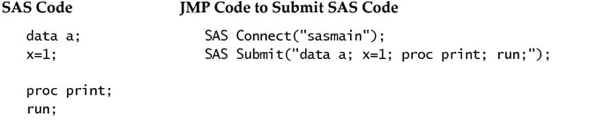
You can submit SAS code directly from JMP to the currently active SAS server. If the submitted SAS code generates SAS Listing output, that output is automatically retrieved from the SAS server and displayed in JMP. Also, the generated SAS Log is retrieved, and, if there are any errors in the submitted code, the SAS Log is automatically displayed in the SAS Log window.

All analyses in JMP are run natively within JMP without any dependency on the SAS System. The SAS code that JMP generates is intended to enable you to perform a separate but similar analysis in the SAS System after the initial JMP analysis, or to score new observations in the SAS System using a model that was fit within JMP.

Figure 3.21 SAS Code Submission Example

The following JMP platforms generate SAS code:

•Standard Least Squares - PROC GLM

•REML - PROC MIXED

•Stepwise - PROC GLM

•Nominal and Ordinal Logistic - PROC LOGISTIC

•GLM - PROC GENMOD

•Time Series (ARIMA and TFM) - PROC ARIMA

•Neural - SAS Data Step scoring code

•Partition (Decision Tree, Bootstrap Forest, Boosted Tree) - SAS Data Step scoring code

Note: Use the JSL function As SAS Expr( formula ); to turn any prediction formula into an expression that can be used in a SAS Data Step. See the JSL Syntax Reference.

To run SAS code directly from JMP

1.Either open an existing SAS program using File > Open, or create a new SAS program. (Create a new SAS program by selecting File > SAS > New SAS Program and typing in the SAS code.)

2.Click theSubmit to SASicon.

You can also right-click in the Program Editor window and select Submit to SAS. The menu item also includes the name of the active SAS server that the SAS code will be submitted to.

You can also press the F8 key (press COMMAND-SHIFT-R on Macintosh).

To run SAS code using a JSL script

Write and run a JSL script that uses either the SAS Submit or SAS Submit File JSL functions. For more information about writing JSL scripts that submit SAS code, see the Scripting Guide.

To view the SAS Listing output

If the submitted SAS code generates SAS Listing (textual) output, that output is automatically be displayed in a SAS Output window when the job is completed. If you need to view the SAS Listing output again later in the JMP session, select File > SAS > Open SAS Output Window. The SAS Output Window retains the listing output from the previous 25 submits to the active SAS server.

To view the SAS log

If the submitted SAS code contained errors, the SAS Log window for the active SAS server is automatically opened, displaying the SAS Log for the job. However, you can view the SAS Log for the most recent 25 submits to the active server at any time by selecting File > SAS > Open SAS Log Window.

If you prefer that SAS Log information is appended to the JMP log after a submit completes:

1.Select File > Preferences (Windows) or JMP > Preferences (Macintosh).

2.Open the SAS Integration category.

3.In the Show SAS Log section, selectJMP Lograther thanSeparate Window.

Also, in the Show SAS Log section, you can set whether the SAS Log should be displayed Always, Never, or On Error (the default).

Generate ODS Results

The SAS Output Delivery System (ODS) is a powerful mechanism for generating reports in HTML, RTF, PDF, and other formats. ODS output is generally much more attractive and customizable than plain-text SAS Listing output. You can set your submitted SAS code generate ODS results rather than SAS Listing output using Preferences.

To generate ODS results from your submitted SAS code

1.Select File > Preferences (Windows) or JMP > Preferences (Macintosh).

2.Open the SAS Integration category and find the large SAS Submit Options group, as shown inFigure 3.22.

Figure 3.22 SAS Submit Options in Preferences

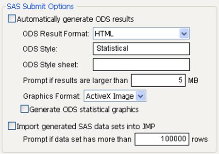
3.Select theAutomatically generate ODS resultsoption.

4.From theODS Result Formatlist, select the format in which to generate the ODS results:HTML,PDF,RTF, or aJMPreport.

5.(Optional) You can use other options to specify a style or style sheet to format the results or set the format for generated graphics. For more details, see“SAS Integration”in the “JMP Preferences” chapter.

Performing the previous steps causes JMP to generate additional SAS code, including an ODS statement, that is wrapped around the SAS code that you submit. The SAS code that you submit then automatically generates ODS results in the specified format. Those results are downloaded to your computer and displayed either within JMP, when possible, or in an appropriate external application.

Retrieve Generated SAS Data Sets

SAS code that you submit might generate SAS data sets. You can have them automatically imported into JMP for further analysis.

1.Select File > Preferences (Windows) or JMP > Preferences (Macintosh).

2.Open the SAS Integration category.

3.Select theImport generated SAS data sets into JMPoption.

Export JMP Data Tables to SAS

You can export JMP data tables to a SAS Workspace Server.

1.Connect to the SAS Workspace Server.

2.Open the file that you want to export.

3.SelectFile > SAS > Export Data to SAS.

If necessary, you are connected automatically using your profile’s user name and password.

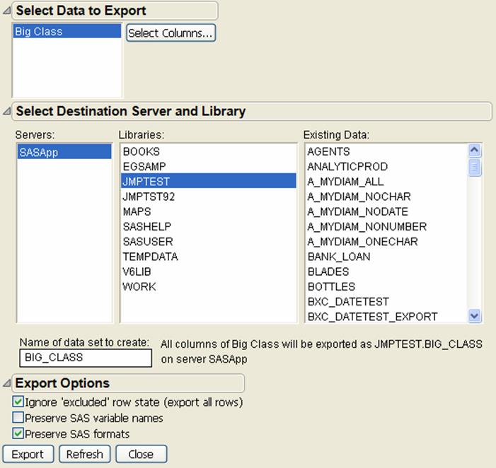
4.Select the data table that you want to export to SAS from the list of open data tables under Select Data to Export.

Figure 3.23 Export Data to SAS

5.(Optional) To export only some of the columns in the data table, clickSelect Columns. See“To select columns to export”for details.

6.Select the Destination Server.

7.Select the Library.

Tip: If your libraries do not appear, see “Show Libraries in the Export Data to SAS Window”.

A list of the data sets in the library appears.

8.Enter the name as you want it to appear in the SAS library.

9.(Optional) Set the export options that you want to use. See“Export Options”for details.

10.ClickExport.

To select columns to export

1.To export only some of the columns in the data table, click Select Columns.

2.In the window that appears, select the columns to export and clickAdd.

3.When all the columns have been added to the Selected Columns list, clickOK.

Export Options

The available export options are as follows:

Ignore ‘excluded’ row state (export all rows)

Select this option to export all rows in the data table. Deselect this option to export only those rows that are not excluded. This option is on by default.

Preserve SAS variable names

This option is useful for data tables that were imported originally from SAS. When importing a SAS data set, the original SAS variable name is saved in a column property for each column. Select this option to use the SAS variable name for each column when exporting to SAS. Deselect this option to export the JMP variable names. This option is off by default.

Preserve SAS formats

This option is useful for data tables that were imported originally from SAS. When importing a SAS data set, the original SAS format and informat is saved in a column property for each column. Select this option to use the SAS format and informat for each column when exporting to SAS. Deselect this option to export the JMP formats instead. This option is on by default.

Show Libraries in the Export Data to SAS Window

If your libraries do not appear in the Export Data to SAS window, define the library in one of the following ways:

•Using JSL, submit code to the SAS server. The code defines a library using a libref command.

•Define an autoexec.sas file that runs a snippet of SAS code every time SAS is invoked. This creates the same librefs every time you connect to SAS. For details about autoexec.sas files, see the SAS documentation.

Libraries that are defined in metadata (such as libraries defined in the SAS Management Console under the Data Library Manager) cannot be accessed from the Export Data to SAS window.

Build SQL Queries in Query Builder

Query Builder is the preferred method for selecting and importing data from an SQL database without writing SQL statements. You can preview the data before importing it into a data table. Share your queries so that other users can customize and run the queries.

Query Builder provides an alternative to writing your own queries using the File > Database > Open Table feature. However, you can also start building a query in Query Builder and then add your own SQL statements.

SAS Query Builder is also available for querying SQL databases on SAS servers. See “Open SAS Data Sets with SAS Query Builder” for details.

Note: Database table names that contain the characters $# -+/%()&|;? are not supported.

Connect to an SQL Database

Set up the ODBC connection through the Windows Control Panel or inside JMP.

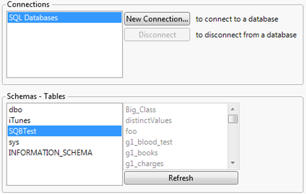
1.Select File > Database > Query Builder to display the Select Database Connection window.

The Connections box lists data sources that you connected to in the current JMP session.

2.If the desired data source isnotlisted in the Connections box, clickNew Connectionto choose a data source. The method of choosing a data source depends on your operating system and the ODBC driver. See“Connect to a Database”for details.

3.Select a table or schema from the Schemas - Tables box and clickNext.

Query Builder examples are based on a table named SQBTest, which contains movie rental data.

Figure 3.24 Select the Database Schema

Select Tables from an SQL Database

After connecting to the SQL database, select the tables that you want to query. Either select a primary table or join several tables to query them all.

By default, JMP attempts to join tables based on key relationships that are assigned in the tables.

•A primary key identifies a column that uniquely describes the data (for example, a customer ID number). All rows from the primary table are included in your query.

•A foreign key in a secondary table matches the primary key in one of the joined tables. Only matching rows from the secondary table are included in your query.

If there are no keys, data are matched by column name. By default, only matching rows from the secondary tables are included in the query.

This example shows how to join multiple tables. However, you can also build a query using a single table. In this case, joining is not necessary.

1.Select File > New > Database Query, connect to the database, and select the SQBTest schema. (See “Connect to a Database” for details.)

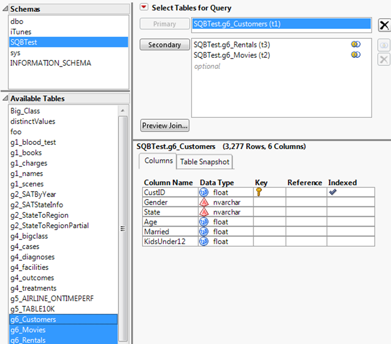
2.In the Select Tables for Query window, selectg6_Customersfrom the Available Tables list, and then clickPrimary.

The Columns tab shows that CustID is the primary key. The data is indexed, which speeds up the query.

3.Selectg6_Moviesandg6_Rentalsfrom the Available Tables list, and then clickSecondary.

The Left Join icon indicates that the tables were automatically joined (Figure 3.25). CustID is the primary key in g6_Customers and matches a foreign key in one of the other tables.

Figure 3.25 shows the completed window.

Figure 3.25 Selecting Primary and Secondary Tables

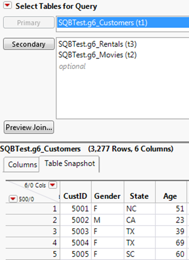
4.Click theTable Snapshottab for each table to preview the data (Figure 3.26).

Figure 3.26 Matched Rows on the Table Snapshot Tab

5.Below the primary and secondary tables, clickPreview Jointo see a preview of the table that was created from the specified joins.

Tips:

•The red X icon next to a secondary table indicates that the table is not joined in the query. Click the Edit Join button to specify the columns to join. If you cannot find columns to join, click the Remove button to remove the table. See “Edit the Conditions for Joining Tables” for details.

•To quickly remove tables that you have added to the query and start the process again, click Start Over in the upper right corner. Click Change Data Source to query a different schema or database.

•To rename a table alias, right-click the table in the Query Builder’s Tables pane and select Change Alias. The alias is updated throughout the query.

Edit the Conditions for Joining Tables

In the Select Tables for Query red triangle menu, Auto join Database Tables is initially selected. JMP automatically joins database tables based on key relationships or matching column names.

If there are no keys, or when column names do not match, click the Edit Join button to specify the columns to join.

To edit the conditions for joining tables

1.Select File > New > Database Query, connect to the database, and select the SQBTest schema. (See “Connect to a Database” for details.)

2.In the Select Tables for Query window, selectg1_booksas the Primary table andg1_chargesas the Secondary table.

The red X icon next to the secondary table indicates that the table is not joined in the query.

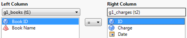
3.Selectg1_chargesin the Secondary table pane and click theEdit Joinbutton.

The Edit Join window appears.

4.In the Left Column list, selectg1_books.

5.SelectBook IDfrom the Left Column box.

6.SelectIDfrom the Right Column box.

7.Make sure that the equal sign is selected between the two boxes.

Figure 3.27 The Edit Condition Window

8.ClickNext.

The Edit Join window shows that non-matching rows from g1_books will be included in the data table. Rows that are only in g1_charges will be omitted.

To do a full join and import all rows, you would select Include non-matching rows from g1_charges.

9.ClickOK.

Note: The OK button is unavailable until all of the secondary tables are joined.

To prevent tables from joining automatically

•Deselect Auto join Database Tables from the Select Tables for Query red triangle menu above the primary table.

•If you frequently query large databases, deselect Automatically join tables added to a query in Preferences > Query Builder to prevent memory issues.

Build the SQL Query

After selecting database tables, you either import the data or build a query. Query Builder enables you to interactively create the database query rather than write SQL expressions.

After selecting database tables (and joining them if necessary), click Build Query to open the Query Builder window. You can continue to refine the query by selecting which columns to include and specifying criteria for sampling and filtering. You can also save the query to edit and run again later.

The columns from all data tables appear in the Available Columns list. Prefixes such as t1 and t2 (also called aliases) associate each column with the corresponding data table.

To skip the Query Builder step and import all data, click Import Now instead.

Select Columns from the Database Table

Suppose that you want to view movie rentals by movie genre, rating, and demographic data such as marital status and age.

1.Select File > New > Database Query, connect to the database, and select the SQBTest schema. (See “Connect to a Database” for details.)

2.In the Select Tables for Query window, selectg6_Customersand clickPrimary.

3.Selectg6_Moviesandg6_Rentalsand clickSecondary.

4.ClickBuild Queryto show the Query Builder window.

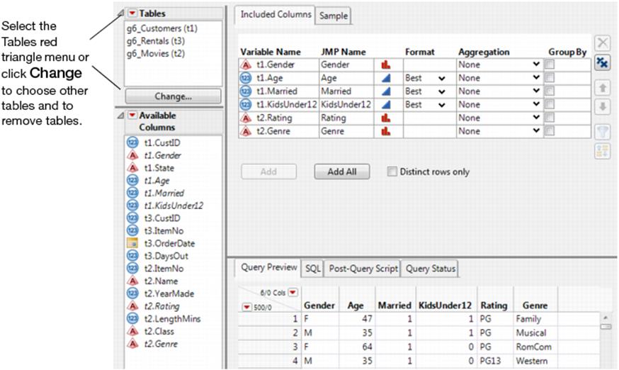
5.In the Available Columns box, selectt1.Gender,t1.Age,t1.Married,t1.KidsUnder12,t2.Rating, andt2.Genre.

6.ClickAddon the Included Columns tab.

Figure 3.28 Selected Columns

7.Select theSQLtab below the columns to view the SQL statements for your query. This code is saved as a data table property after you run the query.

8.ClickSavein the lower right corner.

Your work is saved as g6_Customers.jmpquery, which you can open later to return to this point or to run the query.

9.ClickRun Queryto import the data.

The data table includes the following scripts:

‒Run the Source script to reconnect to the database.

‒Run the Modify Query script to open the query in Query Builder.

‒Run the Update From Database script to re-import and refresh the data.

Tips:

•To rename a column, double-click the JMP Name in the Included Columns tab and enter a new name.

•To rename an alias, right-click the table in the Tables pane and select Change Alias. You can also right-click the table name in the Select Tables for Query window to rename the alias. The change appears throughout the query. Aliases are not case sensitive.

•To view the number of records being read during the query, deselect the preference or view the Query Status tab. The query runs in the background unless you deselect Run queries in the background when possible from the Query Builder ODBC preferences. You can also check the progress of all ODBC queries by selecting View > Running Queries.

Note: For SAS Query Builder, all queries run in the foreground.

•Deselect Update preview automatically if the preview loads too slowly. Click Update below the Query Preview tab to update the data view. Consider changing the Preview options in the JMP Query Builder preferences if you frequently work with large databases.

•To omit duplicate rows from the database, select Distinct rows only on the Included Columns tab.

Group the Common Values

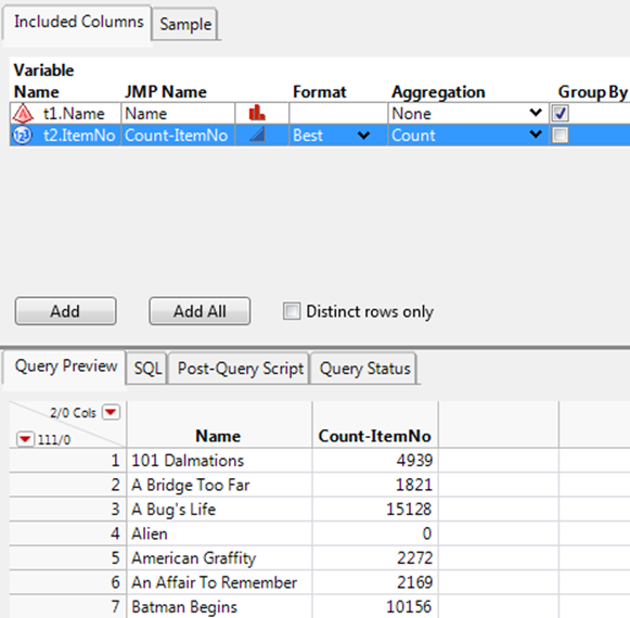
You can combine (or group) common values in a column before importing the data into JMP. To group common values, select an Aggregation function to determine how the common values are calculated.

Suppose that you are interested in the number of times a specific movie was rented. In this example, the count for each item number is calculated, and common movie values are grouped into single rows.

1.Select File > New > Database Query, connect to the database, and select the SQBTest schema. (See “Connect to a Database” for details.)

2.In the Select Tables for Query window, selectg6_Moviesas the Primarytable andg6_Rentalsas the Secondary table.

3.ClickBuild Queryto show the Query Builder window.

4.In the Available Columns box, selectt1.Nameandt2.ItemNoand clickAdd.

5.Selectt2.ItemNoand selectCountfrom the Aggregation list.

The Group By check box is selected for t1.Name (Figure 3.29). All instances of a specific movie name will be grouped into one row.

Figure 3.29 Grouped Columns

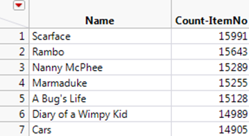
6.ClickRun Queryto import the data.

7.In the data table, right-click theCount-ItemNocolumn and selectSort > Descending.

Scarface was rented most frequently (Figure 3.30).

Figure 3.30 Sorted Count-ItemNo Column

Tips:

•To clear the grouped rows, select None from the column’s Aggregation list.

•The DISTINCT Aggregation functions show only rows that contain distinct values. Rows with duplicate values are omitted. These functions are useful when a database contains many duplicate values.

Import a Sample of the Data

With large databases, consider sampling the data. Sampling returns a subset of rows and decreases the query time. The database query runs, and a smaller portion of data are imported based on options that you select on the Sample tab.

Sampling methods differ based on the database vendor.

•SQL Server supports block sampling by default. A block sample takes an entire page of rows (such as all rows on pages 1 and 5). If you select 1,000 rows, approximately 1,000 rows are imported.

•Oracle and other databases support row sampling. If you select 5,000 rows, between 4,800 and 5,200 rows per sample are typically imported, based on how Oracle cycles through the data.

For major database vendors, JMP detects the capabilities and provides vendor-specific options when possible. Features that are unsupported by the vendor are unavailable on the Sample tab.

Suppose that you want to import a sample of the data. In this example, you select the first 5,000 rows.

1.Select File > New > Database Query, connect to the database, and select the SQBTest schema. (See “Connect to a Database” for details.)

2.In the Select Tables for Query window, selectg6_Rentalas the Primarytable andg6_Moviesas the Secondary table.

3.ClickBuild Queryto show the Query Builder window.

4.Click theAdd Allbutton on the Included Columns tab.

5.Click theSampletab and selectSample this result set.

6.SelectRandom N Rowsand type 5,000.

In the Sample By area, Blocks or Pages is the only option based on which type of sampling the database supports.

7.ClickRun Queryto import the data.

The new data table consists of approximately 5,000 rows. With block or page sampling, you might get a sample of 4,900 rows one time and 5,600 rows the next time.

Tip: To re-create the same sample set each time you run a query, set the Seed value to any positive integer up to 64,000. Suppose that you want to query movie rentals by gender. Type 1 as the Seed value and run the query. The distribution of male customers in the results is low. Type 2 as the Seed value and run the query again. Repeat this process to find the Seed value that results in a similar distribution of males and females.

Select Filters to Import a Subset of the Data

Add filters to import a subset of values from the selected filters into the data table. In this example, import data for age 30 and over customers, and movies in the Musical genre. You also enable users to apply their own filters when they run this query.

Note: For most columns, the filter is a check box list by default. For columns that contain over 1,000 levels, the Like filter is automatically selected.

1.Select File > New > Database Query, connect to the database, and select the SQBTest schema. (See “Connect to a Database” for details.)

2.In the Select Tables for Query window, selectg6_Rentalsfrom the Available Tables list, and then clickPrimary.

3.Selectg6_CustomersandG6_Moviesand then clickSecondary.

4.ClickBuild Queryto show the Query Builder window.

5.In the Available Columns box, selectt2.Gender,t2.Age, andt3.Genre, and then clickAddon the Included Columns tab.

6.Select all columns on the Included Columns tab and click theAdd Selected Items to Filtersbutton.

Filters for the columns appear in the Filters outline.

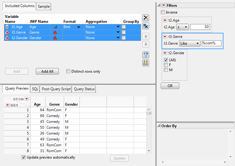
7.Set the t2.Agefilter to ≥ 30.

8.From the t3.Genre red triangle menu, select Like, type%com%, and pressEnter.

The % wildcards match any number of characters before and after “com”. On the Query Preview tab, notice that movies in both the RomCom and Comedy genres are shown (Figure 3.31).

Figure 3.31 Selecting Filters

9.In the Filters red triangle menu, selectAll Prompt on Run.

Users who run the query can customize the filters.

10.ClickRun Query.

11.In the Query Prompts window, clickOKto apply the preselected filters and import the data.

Import Matching Data from an Existing Data Table

You can also select rows from an open data table that match a column in your query. Consider a database of airline data. The database includes data such as flight duration and tail number. You also have a data table that includes tail number data. Use the Match Column Values filter to import only data for matching tail numbers.

1.Select Help > Sample Data Library and open Air Traffic.jmp.

2.SelectFile > New > Database Query, connect to the database, and select theSQBTestschema. (See“Connect to a Database”for details.)

3.In the Select Tables for Query window, selectg5_AIRLINE_ONTIMEPERFfrom the Available Tables list, and then clickPrimary.

4.ClickBuild Queryto show the Query Builder window.

5.ClickAdd Allon the Included Columns tab.

6.Selectt1.TailNumon the Included Columns tab and click theAdd Selected Items to Filtersbutton.

7.From thet1.TailNumred triangle menu in the Filters column, selectFilter Type, and then selectMatch Column Values.

8.SelectAir TrafficbelowMatch values from table.

9.Select theTail Numbercolumn and then selectAll rows (38,118)from the list.

The data view on the Query Preview tab updates to show the filtered values.

10.ClickRun Queryto import the data.

The data table includes only data for rows that are in the Tail Number column.

Write a Custom Expression to Import a Subset of the Data

In addition to selecting filters to subset the data, you can write custom SQL expressions.

1.Select the columns that you want to filter (described in “Select Filters to Import a Subset of the Data”).

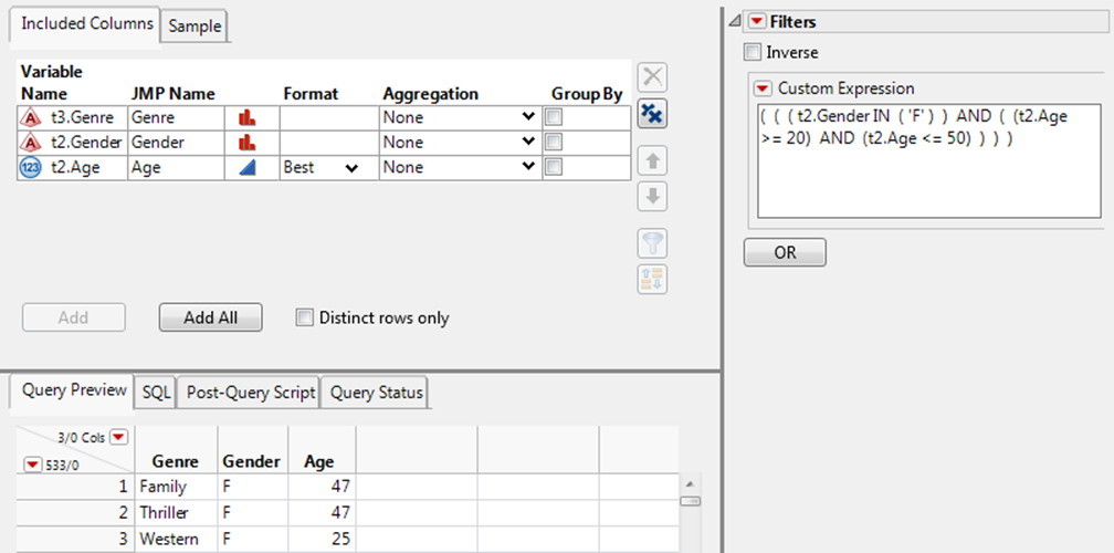
2.From the Filters red triangle menu, selectAdd Custom Expression.

3.Type the following text in the Custom Expression box:

( ( ( t2.Gender IN ( 'F' ) ) AND ( (t2.Age >= 20) AND (t2.Age <= 50) ) ) )

4.Click outside the Custom Expression box to update the Query Preview tab (Figure 3.32).

Figure 3.32 Writing a Custom Filter Expression

Sort the Selected Data

You can sort the rows in specific columns by values to control how the data appear in the data table. In this example, you sort the Married column in descending order and sort the data by Married and then Rating.

1.Select File > New > Database Query, connect to the database, and select the SQBTest schema. (See “Connect to a Database” for details.)

2.In the Select Tables for Query window, selectg4_bigclassas the Primary table.

3.ClickBuild Queryto show the Query Builder window.

4.On the Included Columns tab, clickAdd All.

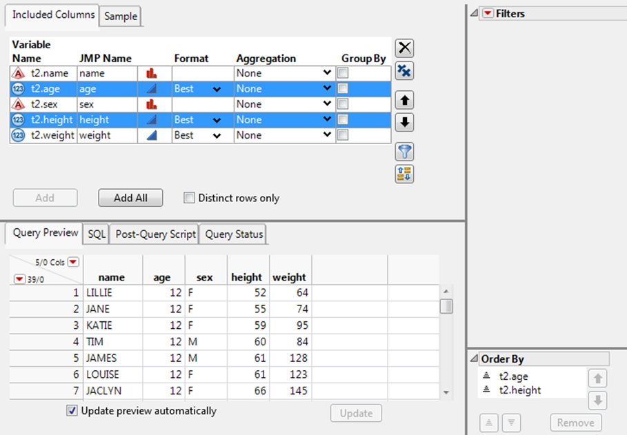
5.Selectt1.ageandt1.heightand click theOrder by the Selected Itemsbutton.

The columns appear in the Order By outline in the right column.

The columns are sorted by age first (youngest to oldest) and then height (shortest to tallest).

Figure 3.33 Selecting the Order By Columns

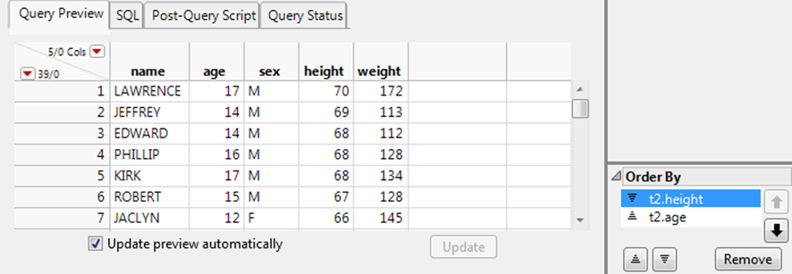
6.In the Order By outline, selectt1.heightand then click theSort the values in descending orderbutton below the columns.

The height column is sorted from tallest to shortest.

7.Selectt1.heightand click theMove the Selected Items Up in the Listbutton.

The height column is sorted first. Values in the age column are sorted within each level of height. For a height of 68, age is sorted from 14 to 17.

Figure 3.34 Result of Reordering Columns

View the Query Status

On the Query Status tab, view the status of a query as it runs in the background. The query name, SQL statements, and number of processed records appear. You can stop a query at any time and view only the processed records. To view background queries from other JMP windows, selectView > Running Queries. The status details are unavailable if you deselect Run queries in the background when possible from the Query Builder preferences.

Note: For SAS connections in Query Builder, all queries and query previews run in the foreground.

Write a Post-Query Script

On the Post-Query Script tab, write a JSL script that runs after you run the query. For example, you might want to import the data and then create a distribution.

Distribution( Column( :age, :gender ) );

This script is part of the Source script in the final data table.

Save and Run the Query

Save your query as a .jmpquery file to modify or run the query later. You are prompted to enter the password if the server connection string does not specify it. The .jmpquery file can also be opened and run by a JSL script.

After you build a query, click Save in the lower right corner to save the settings as a .jmpquery file. Clicking Save again overwrites the file with your latest changes.

Note: The .jmpquery file contains database login information. You must have set up the database connection before running the query. See “Connect to a Database” for details.

Open the Selected Data in JMP

After you specify the columns and data to import, click Run Query to open the data in a data table. The SQL statements are saved as a table variable. The following scripts are available:

Source

Runs the query.

Modify Query

Opens the query in Query Builder, where you can change which columns and data are imported and further customize the query.

Update From Database

Connects to the database to refresh the data and then run the query.

Query Builder Red Triangle Options

The Query Builder red triangle menu provides scripting and custom SQL options. The modify and run scripts are always automatically saved in the final data table.

Copy Modify Script

Copies a script to the computer’s clipboard that lets you modify the query.

Copy Run Script

Copies a script to the computer’s clipboard that lets you refresh the data and run the query.

Save Modify Script to Script Window

Saves the Modify Query script to the script window.

Save Run Script to Script Window

Saves the Update From Database script to the script window.

Convert to Custom SQL

Shows the query statements in a new script editor window. You must remove prompting filters before selecting this option.

When you save the query from the Custom SQL window, the custom SQL is saved. Interactive components that were present before you customized the query are not saved. Revert to Interactive is also unavailable on the red triangle menu.

Revert to Interactive

Displays the interactive query in the Query Builder window. Changes that you made on the Custom SQL tab are not saved when you revert.

Write SQL Statements in Query Builder

Query Builder enables you to interactively create SQL queries without writing SQL statements. You can also build a query in Query Builder and then add custom statements to the query.

1.Select File > New > Database Query, connect to the database, and select the SQBTest schema. (See “Connect to a Database” for details.)

2.In the Select Tables for Query window, selectg6_Rentalsas the Primary table.

3.Selectg6_Moviesandg6_Customersas the Secondary tables.

4.ClickBuild Queryto show the Query Builder window.

5.Click theAdd Allbutton on the Included Columns tab.

6.From the Query Builder red triangle menu, selectConvert to Custom SQLand clickOK.

The SQL that Query Builder generated appears on the Custom SQL tab.

7.Click before the semicolon and type the following SQL statement:

WHERE ( ( ( t2.Gender IN ( 'F' ) ) AND ( (t2.Age >= 20) AND (t2.Age <= 50) ) ) )

8.ClickRun Queryto import the data into JMP.

The data table scripts include the custom query.

Note: If you select Revert to Interactive from the red triangle menu, the changes that you made on the Custom SQL tab are not saved. If you save the custom query and reopen it, Revert to Interactive is not available.

See “Structured Query Language (SQL): A Reference” for a brief primer of SQL statements.

Import Data from a Database

You can import data from a database if you have an ODBC (Open Database Connectivity) driver for the database and then save the data back to the database.

This section describes how to connect to a database and import the data. Refer to “Build SQL Queries in Query Builder” for details about interactively building queries.

Note: Database table names that contain the characters $# -+/%()&|;? are not supported.

Connect to a Database

Your operating system provides an interface for JMP to communicate with databases using ODBC data sources. Create and configure data sources with operating system software. For example, on Windows 7, use Control Panel > System and Security > Administrative Tools > Data Sources (ODBC); on the Macintosh, use Applications > Utilities > ODBC Manager.

After you create the data source in the operating system software, follow these steps to connect to the database in JMP.

1.Select File > Database > Open Table. The Connections box lists data sources that you have connected to in the current JMP session.

2.ClickNew Connection.

3.(Windows) In the Select Data Source window (Figure 3.35), click the Machine Data Source tab, select the data source, clickOK, enter the user name and password, and then clickOK.

(Macintosh) In the Choose DSN window, select the data source, enter the user name and password, and then click Choose DSN.

Figure 3.35 Select a Data Source (Windows)

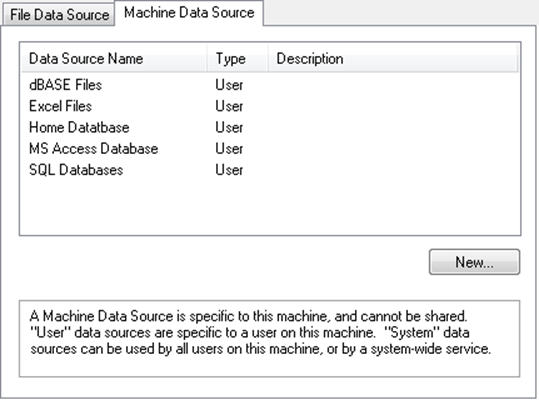
The new connection is shown in the Database Open Table window.

Open Data from a Database

After you connect to the ODBC database and select a table to import, the data is opened in a data table. Several table scripts are included in the data table.

•Run the Source script to reconnect to the database.

•Run the Update from DB script to re-import and refresh the data.

•Run the Save to DB script to save the data table to the database. The existing data in the database is replaced. This script might contain the user name and password. There is a JSL-only preference that can be set to prevent including this possibly sensitive information. See the Scripting Guidefor more details.

To import data from a database

1.Select File > Database > Open Table.

The Database Open Table window appears (Figure 3.36).

2.If you are already connected to the database, select it in the Connections box. Follow the steps in“Connect to a Database”.

The Connections box lists data sources to which JMP is connected. The Schemas - Tables box lists schemas for those databases that support them.

Figure 3.36 Database Open Table Window

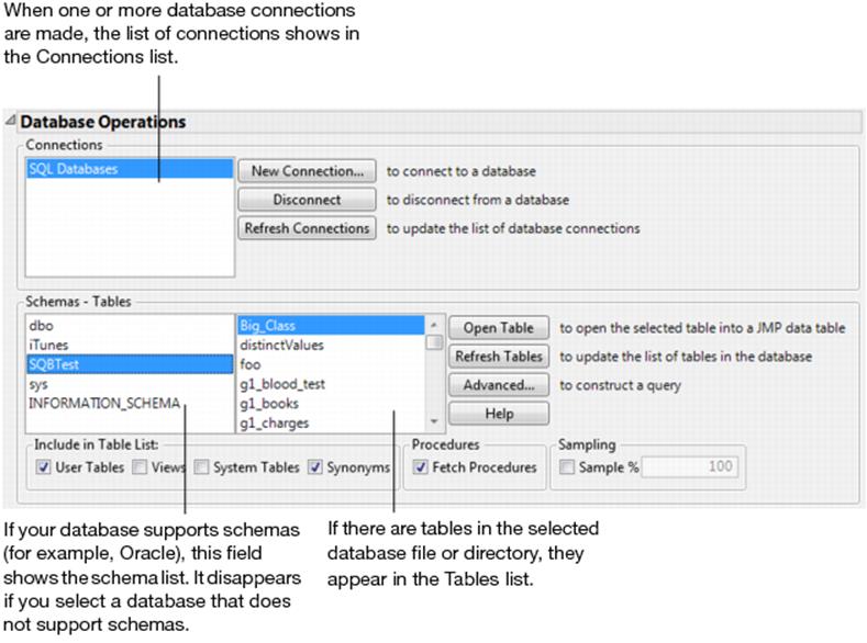
Note: The Fetch Procedures check box is disabled if the ODBC driver does not support fetching procedures.

3.If the desired data source isnotlisted in the Connections box, clickConnectto choose a data source. The method of choosing a data source depends on your operating system. Select a data source and clickOK.

4.Select the desired data source in the Connections box. The tables list in the Tables box updates accordingly. The update might take a several seconds, depending on the number of tables and the speed of the connection to the database. If your database supports schemas, tables are loaded for the first schema in the list, and on other schemas as you click on them.

5.Control which tables are listed by choosing the options in theInclude in Table Listgroup of check boxes. Different drivers interpret these labels differently. Your options are as follows:

User Tables When clicked, displays all available user tables in the Tables list. User tables are specific to which user is logged on to the computer.

Views When clicked, displays “views” in the Tables list along with all other file types that can be opened. “Views” are virtual tables that are query result sets updated each time you open them. They are used to extract and combine information from one or more tables.

System Tables When clicked, displays all available system tables in the Tables list. System tables are tables that can be used by all users or by a system-wide service.

Synonyms When clicked, displays all available ORACLE synonyms in the Tables list.

Sampling Enter the percentage of rows that you want to appear in the list of tables. Selecting this option speeds up queries in large databases. JMP uses the sampling method supported by the database. The check box is unavailable when the database does not support sampling.

6.Select the desired table from the Tables list.

Note: If you are connected to a dBase database, select the database folder to which you would like to connect. Individual files are grayed out and cannot be selected.

7.ClickOpen Tableto import all the data in the selected table, or clickAdvancedto specify a subset of the table to be imported. Some databases require that you enter the user ID and password to access the data.

You might see a short delay when opening large tables. To see the status of all active ODBC queries, select View > Running Queries.

Write SQL Statements to Query a Database

You can use Structured Query Language (SQL) statements to control what you import from a database. When you open a database file in JMP, you are actually sending an SQL statement to the database. By default, this statement gets all files and records in the database table. In some cases, this is too much data. When you are interested only in a subset of the table’s data, you can customize the SQL request to only request the data that you want. After you execute an SQL query, the code for the query is stored in the data table in the SQL table variable.

This section describes how to write SQL statements to retrieve data. To interactively query data without writing SQL statements, use Query Builder. You can also start creating a query in Query Builder and then add your own SQL. See “Write SQL Statements in Query Builder” for details.

1.Select File > Database > Open Table.

The Database Open Table window appears (Figure 3.36).

2.Connect to the database if necessary or select an existing database connection. Follow the steps in“Connect to a Database”.

The Connections box lists data sources to which JMP is connected. The Schemas - Tables box lists schemas for those databases that support them.

Note: The SQL Query that you run in this window operates only on the tables and procedures that are displayed in the left panes of the window. Running unrelated SQL here has no results.

3.From the Database Open Table window, click theAdvancedbutton to open specific subsets of a table.

4.Either type in a valid SQL statement, or modify the default statement.Figure shows a default SQLSelectstatement appropriate for the selected file. See“Structured Query Language (SQL): A Reference”, for a description of SQL statements that you can use.

Instead, you can add expressions by clicking the Where button and using the WHERE Clause editor to create expressions. See “Use the WHERE Clause Editor”, for details.

Figure 3.37 Reading All Variables from the Solubility Table Stored in an Excel File

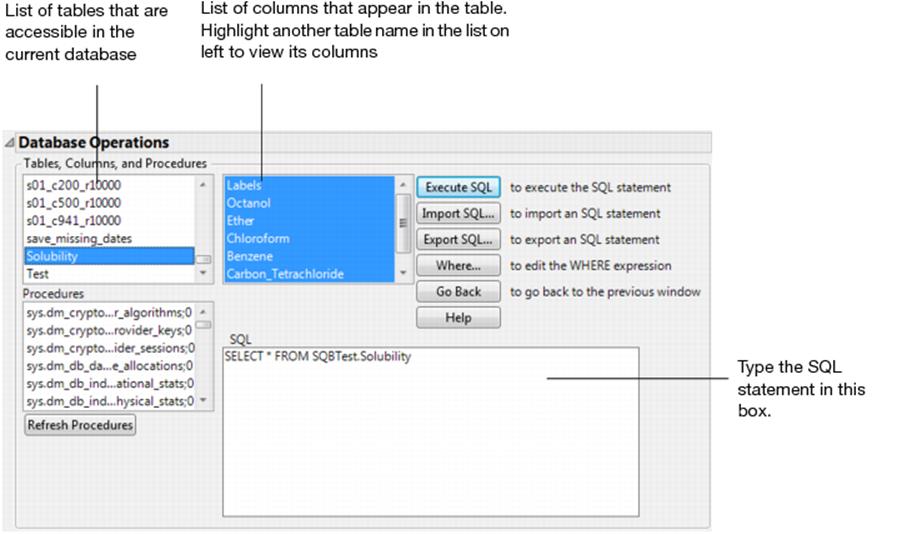
5.ClickExecute SQL. A JMP data table appears with the columns that you selected. The SQL statement becomes an SQL table variable in the JMP data table. (For details, see“Use Table Variables”in the “Enter and Edit Data” chapter.)

6.To see the status of all running queries, selectView > Running Queries.

Note that you can enter any valid SQL statement and click Execute SQL to execute the command. Valid SQL varies with the data source and ODBC driver.

Structured Query Language (SQL): A Reference

The following sections are a brief introduction to SQL. They give you insight to the power of queries, and they are not meant to be a comprehensive reference.

Use the SELECT Statement

The fundamental SQL statement in JMP is the SELECT statement. It tells the database which rows to fetch from the data source. When you completed the process in “Write SQL Statements to Query a Database” with the Solubility.jmp sample data table, you were actually sending the following SQL statement to your data source:

SELECT * FROM "Solubility"

The * operator is an abbreviation for “all columns.” So, this statement sends a request to the database to return all columns from the specified data table.

Rather than returning all rows, you can replace the * with specific column names from the data table. In the case of the Solubility data table example, you could select the ETHER, OCTANOL, and CHLOROFORM columns only by submitting this statement:

SELECT ETHER, OCTANOL, CHLOROFORM FROM "Solubility"

Note: JMP does not require you to end SQL statements with a semicolon.

JMP provides a graphical way of constructing simple SELECT statements without typing actual SQL. To select certain columns from a data source, highlight them in the list of columns (Figure ).

To highlight several rows

•Shift-click to select a range of column names

•Ctrl-click (Windows) or Command-click (Macintosh) to select individual column names.

Note that the SQL statement changes appropriately with your selections.

Sometimes, you are interested in fetching only unique records from the data source. That is, you want to eliminate duplicate records. To enable this, use the DISTINCT keyword.

SELECT DISTINCT ETHER, OCTANOL, CHLOROFORM FROM "Solubility"

Sort Results

You can have the results sorted by one or more fields of the database. Specify the variables to sort by using the ORDER BY command.

SELECT * FROM "Solubility" ORDER BY LABELS

selects all fields, with the resulting data table sorted by the LABELS variable. If you want to specify further variables to sort by, add them in a comma-separated list.

SELECT * FROM "Solubility" ORDER BY LABELS, ETHER, OCTANOL

Use the WHERE Statement

With the WHERE statement, you can fetch certain rows of a data table based on conditions. For example, you might want to select all rows where the column ETHER has values greater than 1.

SELECT * FROM "Solubility" WHERE ETHER > 1

The WHERE statement is placed after the FROM statement and can use any of the following logical operators.

When evaluating conditions, NOT statements are processed for the entire statement first, followed by AND statements, and then OR statements. Therefore

SELECT * FROM "Solubility" WHERE ETHER > -2 OR OCTANOL < 1 AND CHLOROFORM > 0

is equivalent to

SELECT * FROM "Solubility" WHERE ETHER > -2 OR (OCTANOL < 1 AND CHLOROFORM > 0)

Use the IN and BETWEEN Statements

To specify a range of values to fetch, use the IN and BETWEEN statements in conjunction with WHERE. IN statements specify a list of values and BETWEEN lets you specify a range of values. For example,

SELECT * FROM "Solubility" WHERE LABELS IN (’Methanol’, ’Ethanol’, ’Propanol’)

fetches all rows that have values of the LABELS column Methanol, Ethanol, or Propanol.

SELECT * FROM "Solubility" WHERE ETHER BETWEEN 0 AND 2

fetches all rows that have ETHER values between 0 and 2.

Use the LIKE Statement

With the LIKE statement, you can select values similar to a given string. Use % to represent a string of characters that can take on any value. For example, you might want to select chemicals out of the Solubility data that are alcohols, that is, have the OL ending. The following SQL statement accomplishes this task.

SELECT * FROM "Solubility" WHERE LABELS LIKE ‘%OL’

The % operator can be placed anywhere in the LIKE statement. The following example extracts all rows that have labels starting with M and ending in OL:

SELECT * FROM "Solubility" WHERE LABELS LIKE ‘M%OL’

Use Aggregate Functions

Aggregate functions are used to fetch summaries of data rather than the data itself. Use any of the following aggregate functions in a SELECT statement.

Some examples include:

•The following statement requests the sum of the ETHER and OCTANOL columns:

SELECT SUM(ETHER), SUM(OCTANOL) FROM "Solubility"

•This statement returns the number of rows that have ETH values greater than one:

SELECT COUNT(*) FROM "Solubility" WHERE ETHER > 1

•The following statement lets you know the average OCT value for the data that are alcohols:

SELECT AVG(OCTANOL) FROM "Solubility" WHERE LABELS LIKE ‘%OL’

Note: When using aggregate functions, the column names in the resulting JMP data table are Expr1000, Expr1001, and so on. You probably want to rename them after the fetch is completed.

The GROUP BY and HAVING Commands

The GROUP BY and HAVING commands are especially useful with the aggregate functions. They enable you to execute the aggregate function multiple times based on the value of a field in the data set.

For example, you might want to count the number of records in the data table that have ETHER=0, ETHER=1, and so on, for each value of ETHER.

•SELECT COUNT(ETHER) FROM "Solubility" GROUP BY (ETHER) returns a single column of data, with each entry corresponding to one level of ETHER.

•SELECT COUNT(ETHER) FROM "Solubility" WHERE OCTANOL > 0 GROUP BY (ETHER) does the same thing as the above statement, but only for rows where OCTANOL > 0.

When using GROUP BY with an aggregate function of a column, include the column itself in the SELECT statement. For example,

SELECT ETH, COUNT(ETHER) FROM "Solubility" GROUP BY (ETHER)

returns a column containing the levels of ETHER in addition to the counts.

Use Subqueries

Aggregate functions are also useful for computing values to use in a WHERE statement. For example, you might want to fetch all values that have greater-than-average values of ETHER. In other words, you want to find the average value of ETHER, and then select only those records that have values greater than this average. Remember that SELECT AVG(ETHER) FROM "Solubility" fetches the average that you are interested in. So, the appropriate SQL command uses this statement in the WHERE conditional:

SELECT * FROM "Solubility" WHERE ETHER > (SELECT AVG(ETHER) FROM "Solubility")

Save and Load SQL Queries

After constructing a query, you might want to repeat the query at a later time. You do not have to hand-type the query each time you want to use it. Instead, you can export the query to an external file. To do this, click the Export SQL button in the window shown in Figure 3.37. This brings up a window that lets you save your SQL query as a text file.

To load a saved query, click the Import SQL button in the window shown in Figure 3.37. This brings up a window that lets you navigate to your saved query. When you open the query, it is loaded into the window.

Use the WHERE Clause Editor

JMP provides help building WHERE clauses for SQL queries during ODBC import. It provides a WHERE clause editor that helps you build basic expressions using common SQL features, allowing vendor-specific functions. For example, you do not need to know whether SQL uses ‘=’ or ‘==’ for comparison, or avg() or average() for averaging.

In addition, string literals should be enclosed by single quotes (‘string’)rather than double quotes ("string").

To open the WHERE clause editor

1.Connect to a database by following the steps in “Connect to a Database”.

2.From theDatabase Open Tablewindow, click theAdvancedbutton.

3.Click theWherebutton.

USE the WHERE Clause Editor to add any of the following from the work panel: expressions, functions, and terms. They are applied to the highlighted red box.

1.Click the Table Name Browser to select a table. The columns in that table appear in the list.

2.Click the SQL Vendor Name Browser to select the type of SQL that you want to use: GenericSQL, Access, DB2, MySQL, Oracle, SQL Server, or all of the above. Perform an action by clicking a function or operator in the list and selecting an operator from the list that appears.

Note: The following SQL Server data types are not supported: Binary, Geography, and Geometry.

3.Select an empty formula element in the formula editing area by clicking it. It is selected when there is a red outline around it. All terms within the smallest nesting box relative to the place that you clicked become selected. The subsequent actions apply to those combined elements.

4.Add operators to an expression by clicking buttons on the keypad.

5.(Optional) To customize your WHERE clause, select one of the options from the red triangle menu above the keypad:

Show Boxing

Show or hide boxes around the WHERE clause terms.

Larger Font

Increase the font size of the formula.

Smaller Font

Decrease the font size of the formula.

Simplify

Simply the WHERE clause statement as much as possible.

The WHERE clause editor works similarly to the Formula Editor, which is described in the “Formula Editor” chapter.

Figure 3.38 The WHERE Clause Editor

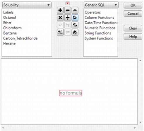
Import Text Files

You can open text files with the extensions .txt, .csv, and .tsv, and the text is converted to a data table. Files with the .dat extension that consist of text are also supported. Text files can be delimited using almost any character, or they can be fixed-width files.

Trailing whitespace and quoted whitespace are removed when you import text files into JMP.

To adjust import settings, choose from one of the following options

•Select File > Preferences > Text Data Files to change the import settings so that JMP determines the best way to structure and format the data table.

•Manually select the import settings as you open the file (described in this section).

•Open the file in the Script Editor, edit the content, and then import the content. This option is helpful when you need to add text delimiters or modify the text.

To import a text file

1.Select File > Open.

2.On Windows, you can set the file type toText Files.

3.Select the text file that you want to open.

For information about the options, see Table 3.3.

Note: On Windows, JMP can open text files in your computer’s default text editor. Select File > Open, and then select All Files (*.*) from the File name list. Select the text file, and then select Use default program to open. Uncheck to open as text.

For details about importing text from a Script window, see “Import Text from the Script Window”.

Text Import Preview Options

When you open a text file that JMP supports, JMP can show a preview of the text before opening the file as a data table. This option lets you manually arrange and format the data. For example, you can specify the end-of-line character or strip quotation marks.

JMP detects the file’s structure and shows options for importing text with either delimiters or fixed width fields. If JMP chooses the wrong file structure, click the Delimited fields or Fixed width fields radio button to import the data as the correct format. (For example, the fixed width window might appear when your file is actually delimited.)

The text import preview options are shown in Figure 3.39 and Figure 3.40.

Figure 3.39 Text Import Preview for Fixed Width Files

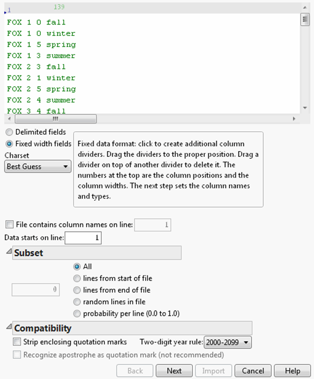
Figure 3.40 Text Import Preview for Delimited Files

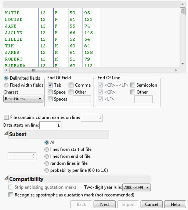
Charset

Select the character set used in the imported file, or let JMP detect the character set. If incorrect characters are displayed in the imported file, open the file again and select another character set.

End of Field

(Available only in the Delimited Import window) Select the check boxes beside the character that marks the end of a field. Alternatively, select the check box beside Other and enter a character if the appropriate character is not listed.

End of Line

(Available only in the Delimited Import window) Select the check boxes beside the character that marks the end of a line (row). Alternatively, select the check box beside Other and enter a character if the appropriate character is not listed. Note that when JMP finds double quotation marks, the delimiter rules change to look for an end double quotation mark. Other text delimiters, including spaces embedded within the quotes, are ignored and treated as part of the text string.

File contains column names on line

Tell JMP where to find data to use as column names. For example, if the column names in your text file are on line (row) 3, select this option and type 3 in the check box. Otherwise, JMP uses the data in the first line of the imported file as the column name in the JMP data table or takes the first line as data.

Data starts on line

Specify the number of the first line that contains data.

Number of Lines

Specify the number of lines (rows) that you want to import.

Strip enclosing quotation marks

Available only on fixed-width imports. Select this check box when you want JMP to remove quotation marks that enclose data in the text file.

Two-digit year rule

Specify how to display dates that have two-digit years. Select the 100-year range in which your dates fall. For example, if the earliest date is 2/2/79, and the year is 1979, select 1970-2069. If the earliest date is 2/2/12, and the year is 2012, select 2000-2099. If dates span centuries, you must recode the dates with four-digit years before importing the data.

Recognize apostrophe as quotation mark (not recommended)

(Available only in the Delimited Import window). Use this option only if your data comes from a nonstandard source that places apostrophes around data fields rather than quotation marks.

When you are finished selecting the settings, click Next. The next window shows each column’s modeling type. To change the default modeling types, do one of the following:

•Click on the data type icon to change the data type from numeric to character. Clicking the icon cycles between the modeling type and exclude. Exclude means that the column is not imported.

•To change a numeric column’s data format, select the format from the red triangle menu.

•Click on the column heading to modify the text.

The top of the Text Import window shows a preview of the text file as it appears when imported into a JMP data file. Click the Import button to import the data.

Figure 3.41 Text Import Preview Window with Column Options

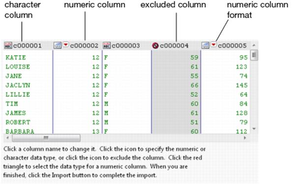
6.When you are finished, clickImportto complete the text import.

Open a Text File in a Text Editing Window

You can open a text file in a Script window, where you edit the text. Then you can import the text as a data table. This feature is helpful when you want to reformat the text before importing it as a data table. For example, you might need to insert the correct delimiters or modify the text.

Another option is opening a JMP add-in definition (.def) file as text and then editing it in a Script window.

To open a text file in a text editing window (Windows)

Files that you recently opened are listed in the JMP Home window. For most files, right-click the text file and select Open as Plain Text to open the file in a text editing window. JMP add-in definition files cannot be opened as plain text from the JMP Home window.

When you are opening the file for the first time, follow these steps:

1.Select File > Open.

2.Do one of the following:

‒To open a JMP add-in definition file as text, select All JMP Files or JMP Add-In Files from the list next to File name. Click the Open button arrow, and then select Open as Plain Text. The file opens in a Script window. Skip the remaining steps.

‒To open other text files, select Text Files from the list next to File name.

Figure 3.42 Select Text Files

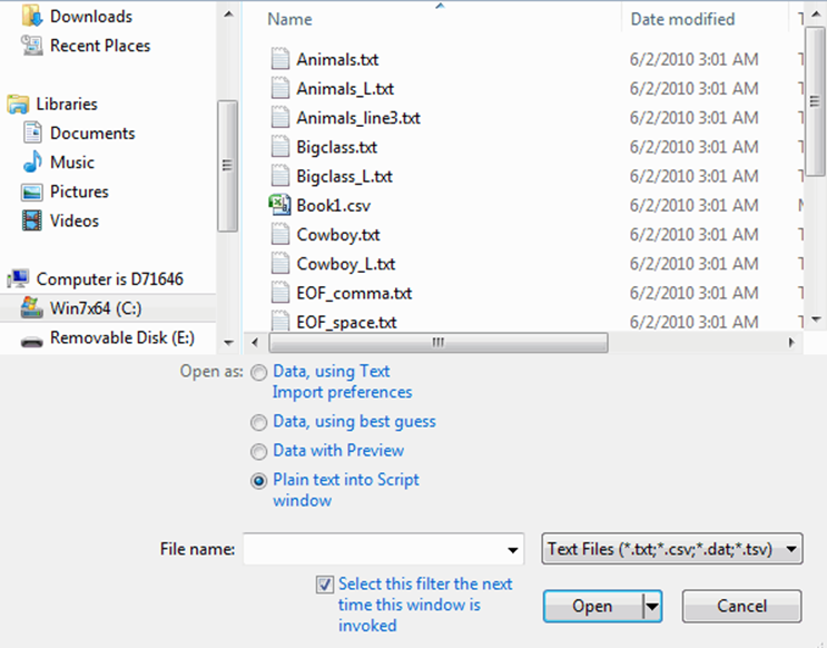
3.(Optional) To set the default option file type toText Files, select the check box besideSelect this filter the next time this dialog is invoked.

4.Select the file.

5.SelectPlain text into Script windownext toOpen as.

6.ClickOpen.

The text appears in a Script window.

To open a text file in a text editing window (Macintosh)

1.Select File > Open.

Figure 3.43 Opening a Text Document on the Macintosh

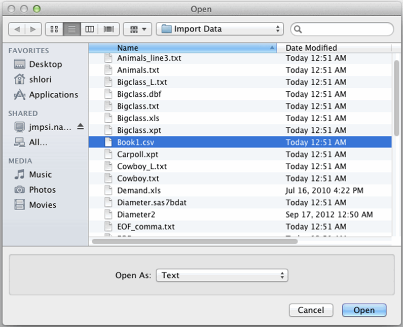
2.Select the file.

3.SelectTextfrom theOpen Aslist.

4.ClickOpen.

The text appears in a Script window.

For details about converting the text to a data table, follow step 3 in “Import Text from the Script Window”.

Import Text from the Script Window

You can import text from the Script window as a data table. The text can be in a table format (for example, from a Microsoft Word document or Web page) or in plain text format. This feature is helpful when you want to reformat the text before importing it as a data table. For example, you might need to insert the correct delimiters or modify the text.

JMP uses the import settings in the preferences to determine how to structure and format the text. Some options include removing quotation marks around text and specifying the rows that contain column headings and data. See “Text Data Files” in the “JMP Preferences” chapter for details.

Note: You can also import an entire web page as a data table. See “Import Remote Files and Web Pages” for details.

This section describes how to import text that you paste into the Script window. For details about opening a text file in the Script window, see “Open a Text File in a Text Editing Window”.

To import text from the Script window

1.Open a new Script window in JMP by selecting File > New > Script (Windows) or File > New > New Script (Macintosh).

2.Copy and paste the text into the Script window.

3.Do one of the following:

‒To import all text from the Script window, select File > Import as Data (Windows) or Edit > Import as Data (Macintosh).

‒To import specific text, select the text, and then select File > Import as Data (Windows) or Edit > Import as Data (Macintosh).

The text is imported into a JMP data table.

Import Remote Files and Web Pages

You import data from Internet sites, intranet sites, FTP sites, or other computers by selecting File > Internet Open. The file paths begin with the Uniform Resource Locators (URLs) http, ftp, or file; a drive letter; or the path to a network drive (relative or absolute).

You also use this feature to import a Web page on a local or network drive as a data table. Once the data table is created, there is a script called Source that you can run to re-import and refresh the data. If you open a web page by selecting File > Open, the page opens in a browser, not as a data table.

SAS stored process reports open in an HTML view. From that view, you can import the file as a data table.

JMP inserts the location of the original data as a note in the data table. For example, the path Z:\example.html is included as a note when you import example.html from the Z drive.

To open a remote file

1.Select File > Internet Open. The window shown in Figure 3.44 appears.

Figure 3.44 Internet Open Window

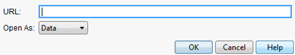
2.Enter the URL.

3.Click the list underOpen As, and select the option that specifies how you would like JMP to display the imported data:

Data Imports the file as a data table.

Web page Opens the web page in a browser. (Select this option to import data generated by web page scripts and server-side requests.)

Text Opens the file in a JMP Script window. In an HTML file, the HTML tags of a .html file are displayed.

4.ClickOK.

One of the following occurs:

‒The file opens as you specified.

‒If you imported a web page as data, a window appears that lists all tables on the page. Select the table or tables that you want to open, and then click OK. Each table opens in a new data table.

‒If you imported a web page as a web page, select File > Import Data as Data Table in the browser. Select the table or tables that you want to open, and then click OK. Each table opens in a new data table.

‒If the file is on an FTP server, the window in Figure 3.45 appears.

Figure 3.45 FTP Login Window

5.For an anonymous account, clickOK. For an authenticated login, enter your user ID and password. The file then opens as you specified.

Note: Some anonymous FTP servers require a user ID. If the data table does not open, try typing either ‘ftp’ or ‘anonymous’ in the User ID text box. Leave the Password text box empty and click OK.

By default, SAS stored processes open reports in an HTML view.

To open a SAS stored process report as a data table

1.In the HTML view, select File > Import Table as Data Table.

A window appears that lists the tables found in the web page.

2.Select the table or tables that you want to import.

3.ClickOK.

Each table is opened as a new data table.

See “Run Stored Processes” for more information about stored process reports.

Tip: If the table you are importing contains images, they are first imported as text. To display the images in your data table, run the automatically generated table script named Load Pictures. A new expression column containing the images is created.

Import SPSS Files

JMP opens SPSS files as data tables and maintains several SPSS features:

•General numeric and character data with minimal formatting are supported.

•SPSS date, datetime, and time formats are supported.

•By default, labels are converted to column headings. When you select this option, and the data contains no labels, the columns are named Column 1, Column 2, and so on.

You also have the option of selecting the conversion method for column headings when opening an SPSS file. The method that you select then overrides the preferences.

To change the default conversion method, select File > Preferences (or JMP > Preferences on Macintosh). On the General page, deselect Use SPSS labels for column names during import. Variable names are then imported automatically as column headings.

•The value labels that you defined in the SPSS file are saved as Value Labels column properties. The value label then appears in each data table cell instead of the original value. For details about Value Label properties, see “Value Labels” in the “The Column Info Window” chapter.

SPSS can assign certain values in a variable to be treated as missing for analyses. For example, the value 64 could be regarded as missing for a Height variable. Then, the calculation of the distribution of height would ignore values of 64. When you import SPSS into JMP, these values are included in the Missing Value Codes column property for the appropriate variable.

At the time of publication, custom currency formats selected in an SPSS file are not maintained on import. In addition, JMP does not read SPSS data that contains double-byte characters, such as non-Unicode Japanese characters.

Note: As with importing other files, you might experience a delay when opening and saving large SPSS files.

To open an SPSS file (Windows)

1.Select File > Open.

2.From the list next toFile name, selectSPSS Data Files (*.sav).

3.Select the SPSS file.

4.(Optional) To specify the column headings, select one of the followingSet JMP column names fromoptions:

‒SPSS Labels creates column headings from SPSS labels.

‒SPSS Variable Names creates column headings from variable names.

5.ClickOpen.

JMP opens the file as a data table.

To open an SPSS file (Macintosh)

1.Select File > Open.

2.Select the SPSS file.

3.(Optional) To specify the column headings, do one of the following

‒Deselect Use SPSS Labels as Headings to convert variable names to column headings.

‒Select Use SPSS Labels as Headings to convert labels to column headings.

4.ClickOpen.

JMP opens the file as a data table.

Import Data from R

JMP provides a scripting interface to R. See the Scripting Guide for details.

Import Data Using the Excel Add-In

The add-in for Excel provides new capabilities to JMP and Excel users on Windows:

•Transfer selected cells in Excel to JMP data tables. See “Transfer Excel Data to a JMP Data Table”.

•Use the JMP Profiler with calculation models in Excel workbooks. The profiler tool is designed to bring the power of the JMP profiler to models residing in Excel worksheets. You do not have to recreate your Excel models in JMP, verify that they are correct, and maintain the model in both JMP and Excel. For more information, see the Profilers book.

Note: During the JMP installation, select the Excel Add-In. This installs the add-in for your version of Microsoft Excel.

•Microsoft Excel 2007, Microsoft Excel 2010, and Microsoft Excel 2013 are supported.

Transfer Excel Data to a JMP Data Table

You can use the JMP Add In for Excel to transfer a worksheet from Excel to the following JMP destinations:

•a data table

•Graph Builder

•Distribution platform

•Fit Y by X platform

•Fit Model platform

•Time Series platform

•Control Chart platform

You can also create models for profiling in JMP. See the Profilers book for details.

To transfer data from Excel to a JMP data table and platform

1.In your Excel worksheet, show the JMP add-in on the ribbon.

2.Click thePreferencesbutton.

3.Accept the defaultData Table Name(File name_Worksheet name) or type a name.

4.SelectUse the first rows as column namesif the first row in the worksheet contains column headers.

5.If you selected to use the first rows a column headers, type the number of rows used.

6.SelectTransfer Hidden Rowsif the worksheet contains hidden rows to be included in the JMP data table.

7.SelectTransfer Hidden Columnsif the worksheet contains hidden columns to be included in the JMP data table.

8.ClickOKto save your preferences.

9.Select the cells to transfer into JMP, including any cells that you want to use as column names.

If you are using cells as column names, they need to be the first rows in your selection.

If only one cell (or no cell) is selected, the entire Excel worksheet is transferred to JMP.

10.Select the JMP destination from the toolbar:

‒Data Table

‒Graph Builder

‒Distribution platform

‒Fit Y by X platform

‒Fit Model platform

‒Time Series platform

‒Control Chart platform

JMP opens, and the selected data is placed in a new JMP data table and the selected launch window appears.

Note: Empty cells are imported as missing data, and dates, numbers, and strings are recognized correctly.

Note: Your JMP windows might be hidden behind your Excel window, especially if you maximize Excel.

For more information about using the various JMP platforms refer to the proper book.

About the JMP Add-In for Excel

The JMP add-in commands are in two groups:

Transfer to JMP

Preferences

Set preferences for transferring data from Excel to JMP.

Data Table

Transfer the selected data in your Excel file to a JMP data table.

Graph Builder

Transfer the selected data in your Excel file to a JMP data table and launch the Graph Builder platform.

Distribution

Transfer the selected data in your Excel file to a JMP data table and launch the Distribution platform.

Fit Y By X

Transfer the selected data in your Excel file to a JMP data table and launch the Fit Y by X platform.

Fit Model

Transfer the selected data in your Excel file to a JMP data table and launch the Fit Model platform.

Time Series

Transfer the selected data in your Excel file to a JMP data table and launch the Time Series platform.

Control Chart

Transfer the selected data in your Excel file to a JMP data table and launch the Control Chart platform.

Profile in JMP

Create/Edit Model

Set up preferences for using the JMP profiler with Excel data.

Run Model

Run the JMP profiler.

Uninstall the Excel Add-In

1.Open the Windows Add or Remove Programs utility (in the Control Panel).

2.SelectJMP Profiler Coreand clickUninstall.

3.SelectJMP Profiler GUIand clickUninstall.

Create New Data Tables

To create a new data table by entering data manually

1.Select File > New > Data Table. This shows an empty data table with no rows and one numeric column, labeled Column 1.

2.Move the cursor onto a cell.

3.Click in the cell. The cursor appears as a line in the cell, as shown inFigure 3.46.

Figure 3.46 A New Data Table

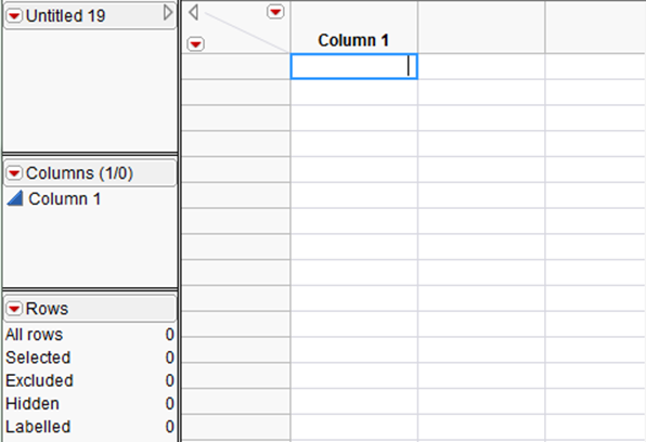
4.Enter a value.

There are several ways to fill a table with values:

•Create new rows and columns and type or paste data into the data grid. (See “Add Rows” in the “Enter and Edit Data” chapter.)

•Construct a formula to calculate column values. (See “Create a Formula” in the “Formula Editor” chapter.)

•Import data from another application. (See “About Importing Data to JMP”.)

•Copy values from another application and paste them into the table.

•Use a measuring instrument to read external measures. See the Scripting Guide for details about data feeds.

•Drag columns from one table to another.

See the “Enter and Edit Data” chapter for details about how to format, edit, and work with data tables.