Using JMP 12 (2015)

Chapter 4. Enter and Edit Data

Perform Basic Data Table Tasks

After you import data into JMP or create a new data table, you can format your data to prepare it for analysis.

This chapter contains the following information:

•Change formatting for numeric values

•Add, delete, and select rows and columns

•Use the Row Editor to navigate within rows and edit rows

•Create scripts that are saved to the data table

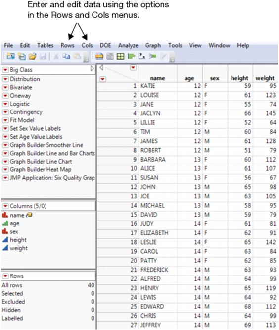
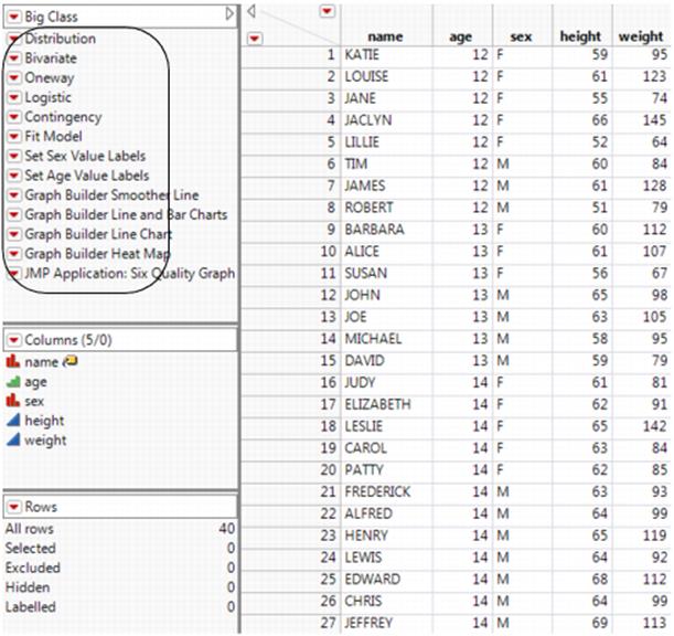
Figure 4.1 The Rows and Cols Menus

Contents

Enter Data

Select Rows

Select Columns

Select Cells

Edit Data

Delete Rows and Columns

Edit or Delete Cells

Edit Column Names

View Patterns of Missing Data

Find and Replace Cell Values

Reorder Columns

Group Columns

Edit Data Tables

Change Table Names

Lock Tables

Compress Tables

Use Table Variables

Create and Save Scripts

Compare Data Tables

Assign Characteristics to Rows and Columns

Hide and Exclude Rows

Exclude Rows and Columns

Hide Rows and Columns

Label Rows and Columns

Assign Colors or Markers to Rows

Create Color Themes

Delete Row Characteristics

Lock Columns in Place

Restructure Data

Enter Data

This section describes how to add rows and columns, fill columns with sequential data, and enter cell formulas.

Add Rows

To add any number of rows to the table

1.Select Rows > Add Rows.

2.Enter the number of rows to add.

3.Specify where to add the new rows (at the start or end of the data table, or after a specific row).

4.ClickOK.

To add a single row to the end of the table

•Below the last row, click anywhere in a cell and begin typing.

•Below the last row, double-click in the empty row number area.

Add Columns

To add new, empty columns

•Double-click the empty space to the right of the last data table column.

•Select Cols > New Column. You can then specify more details about the column. You can also add subsequent columns by clicking Next. See “The Column Info Window”.

•Select Cols > Add Multiple Cols. See “Adding Multiple Columns”.

Note: When you initially create a column, you can choose to fill it with initial data values. See “Fill in Initial Data Values” in the “The Column Info Window” chapter. However, after you modify the cells, this option no longer appears.

Adding Multiple Columns

Using the Add Multiple Columns command to define multiple columns is different from using the New Column command. All of the columns that you add using the Add Multiple Columns window have the same data type. Right-clicking anywhere to the right of the last column in a data table to add multiple columns defaults to After Last Column.

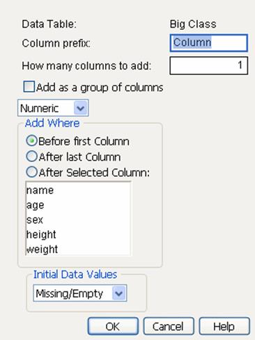
To add multiple columns

1.(Optional) Change the Column prefix.

By default, the new column names are Column 1, Column 2, and so on.

2.Enter the number of columns to add.

3.(Optional) Specify if the columns should be grouped. See“Group Columns”.

4.Select the data type (Numeric, Character, or Row State) for all of the columns. See“About Data Types and Modeling Types”in the “The Column Info Window” chapter.

5.Specify where you want to put the new columns.

6.(Optional) Select initial data values for all of the columns. See“Fill in Initial Data Values”in the “The Column Info Window” chapter.

7.ClickOK.

Figure 4.2 The Add Multiple Columns Window

Tip: To change the modeling type after the columns are created, click on the modeling type icon in the Columns panel and select a different type.

Fill Columns with Sequential Data

To fill columns with a repeating sequence of data or with a continuation of values

1.Create a sequence of data in a column. See Figure 4.3.

Figure 4.3 Example of a Sequence of Data

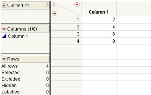
2.Highlight the cells containing the sequenced data. The cells can be in different columns.

3.Right-click the selected cells and select an option underFill.

Fill Options

Repeat sequence to end of table

cells below the selection are filled with repeats of the selected cells.

Continue sequence to end of table

cells below the selection are filled with a continuation of the pattern found in the selected cells. For example, if the selected cells contain the numbers 1 and 2, then the remaining cells are filled with 3, 4, 5, 6, and so on. If the selected cells contain the numbers 2 and 4, then the remaining cells are filled with 6, 8, 10, 12, and so on.

Repeat sequence to

JMP repeats the pattern found in the selected cells to the row number that you specify.

Continue sequence to

JMP continues the pattern found in the selected cells to the row number that you specify.

Enter Cell Formulas

In numeric columns, you can enter cell expressions preceded by an equal sign (=). JMP evaluates the expression and stores the new number as the cell’s value. Unlike column formulas, a cell expression is not stored. Cell expressions can contain operators, constants, and global and column variables.

To enter an expression

1.Click the cell where you want to enter the expression.

2.Type an equal sign (=), and then type the expression. SeeTable 4.1.

3.Press the ENTER key.

Select Rows

To select one entire row

•Click in the empty space that contains the row number.

To select a specific row number

•Select Rows > Row Selection > Go to Row and type in the desired row number.

To select multiple rows

•For continuous selection:

‒Click and drag the cursor over the row numbers.

‒Hold down the SHIFT key and click the first and last rows of the desired range.

‒Hold down the SHIFT key and press the up or down arrow key.

•For discontiguous selection:

‒Hold down the CTRL key and click on each row.

To select or deselect all rows

•To select all rows, select Rows > Row Selection > Select All Rows.

•To deselect all rows, select Rows > Clear Row States.

or

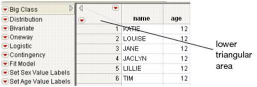
•Hold down the SHIFT key and click the lower triangular area in the upper left corner of the data grid to select. Click again in the same area to deselect all rows. See Figure 4.4.

•To clear all highlighted areas in the data table, press the ESC key.

Figure 4.4 Lower Triangular Area

To select random rows

1.Select Rows > Row Selection > Select Randomly.

2.You can randomly select either a specific number of rows, or a proportion of the total number of rows:

‒Enter a whole number to select that number of rows.

‒Enter a value between 0 and 1 to select that proportion of rows.

For example, enter 10 to select 10 rows. Enter 0.1 to select 10% of the rows.

To invert the row selection

•Select Rows > Row Selection > Invert Row Selection.

To select dominant rows

1.Select Rows > Row Selection > Select Dominant.

2.Choose the column(s) whose values you want to use to determine dominancy.

3.Select the high or low values to dominate by for each column.

4.ClickOK.

Note the following about dominant values and rows:

•A value is dominant over another value if it is higher or lower (based on your specification).

•The Select Dominant option selects each row that is not dominated by any other row. A row dominates another row only if all of its values are dominating the other row’s values.

•The resultant set of rows is called the Pareto Frontier.

To save the current row selection in a new column

1.Select Rows > Row Selection > Name Selection in Column.

2.Type a column name.

3.Label the selected and deselected rows.

4.ClickOK.

To select excluded, hidden, or labeled rows

1.Select Rows > Row Selection.

2.Select from the following options:

‒Select Excluded

‒Select Hidden

‒Select Labeled

Note: For details about excluded, hidden, or labeled rows, see “Assign Characteristics to Rows and Columns”.

Locate Next and Previously Selected Rows

You can locate the next selected row after the current row and cause it to flash by selecting Rows > Next Selected. Similarly, you can locate the previously selected row before the current row and cause it to flash by selecting Rows > Previous Selected.

Each time you select Rows > Next Selected or Rows > Previous Selected, the next or previously selected row is found and flashes. A beep signals when the last selected row is located.

You might want to use this feature when you have selected rows intermittently in a large data set and want to look through the selected rows in the data table.

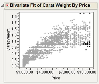
Example of Locating Next and Previously Selected Rows

1.Open the Diamonds Data.jmp sample data table.

2.SelectAnalyze > Fit Y by X.

3.SelectCarat Weightand clickY, Response.

4.SelectPriceand clickX, Factor.

5.ClickOK.

6.SelectTools > Lasso.

If you cannot see the menu bar, place your mouse pointer over the blue bar below the title bar to reveal it.

7.Lasso some of the points near the 10,000 dollar price at the bottom of the plot. SeeFigure 4.5.

8.In the data table, selectRows > Next Selected(or you can press the F7 key).

You can easily navigate through the selected rows to see the data for each.

Figure 4.5 Points Selected

Select Columns

There are several ways to select columns:

•Select columns in the data table itself. See “Select Columns in a Data Table”.

•In a data table that has many columns, select columns by attributes, properties, and statistics in the Columns Viewer. See “Select Columns in the Columns Viewer”.

Select Columns in a Data Table

To select one entire column

•In the data grid, click in the empty space around the column name.

or

•In the Columns panel, click the column name.

To select a specific column number

1.Select Cols > Column Selection > Go to.

2.Enter the column number or name and clickOK.

To select multiple columns

•For continuous selection:

‒Click and drag the cursor over the column name.

‒Hold down the SHIFT key and click the first and last columns of the desired range.

‒Hold down the SHIFT key and press the left or right arrow key.

•For columns that are not next to each other:

‒Hold down the CTRL key and click on each column.

To select or deselect all columns

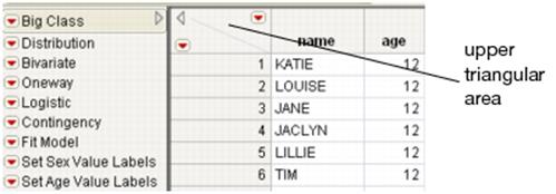
•Hold down the SHIFT key and click the upper triangular area in the upper left corner of the data grid to select. Click again in the same area to deselect all columns. See Figure 4.6.

Figure 4.6 Upper Triangular Area

Tip: To clear all highlighted areas in the data table, press the ESC key.

To invert the column selection

Select Cols > Column Selection > Invert Column Selection. Only the previously deselected columns are selected.

Select Columns in the Columns Viewer

The Columns Viewer helps you quickly select columns by attributes, properties, and statistics, particularly in a data table that has many columns. You can view summary statistics and properties for those columns, view quartiles in the summary statistics, subset the data, and more. And columns in the Columns Viewer window are also linked to the data table columns (Figure 4.7).

Figure 4.7 Linked Columns in the Column Viewer

The Columns Viewer gives you a quick view of data table characteristics. For example, the Summary Statistics report shows which columns contain missing values (Figure 4.8). You can select those columns in the report and then exclude them in the data table.

Figure 4.8 Identify Missing Values

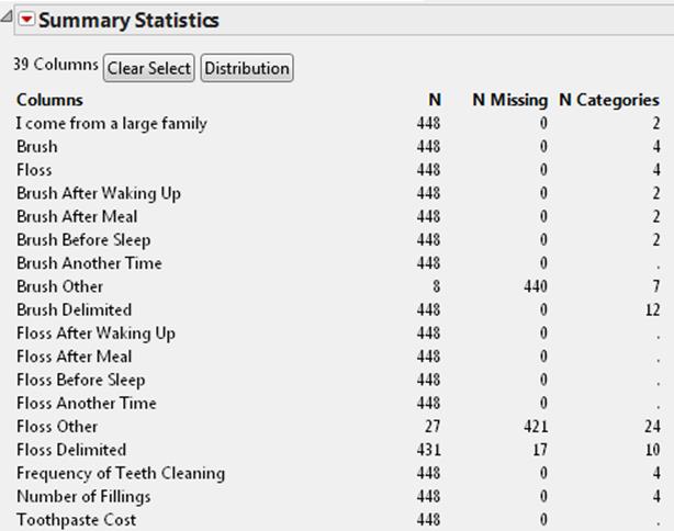
The Summary Statistics report shows the following information:

•the total number of rows (N)

•the number of rows with missing values (N Missing)

•the number of categories (N Categories)

•for continuous data, the Min, Max, Mean, and Std Dev

Other options include the following:

Clear Select

Deselects columns in the data table and in the Columns Viewer. This option ensures that no columns are selected before you begin selecting columns.

Subset

Creates a linked subset data table from the selected columns.

Show Summary

Creates a linked Summary Statistics report for the selected columns. Right-click to select options such as sorting by column or creating a data table. Select Show Quartiles to include lower quartiles, upper quartiles, and interquartile ranges. And to create a linked data table from all columns in the report, select Data Table View from the Summary Statistics red triangle menu.

Find Columns with Properties

Shows a list of column properties in the Columns with Properties report. Select the properties that you want to find and then click OK to create a linked report from all columns. Or you can select columns first in the Select Columns list and then show the list of properties just for those columns.

Tip: Each time you click the Show Summary or Find Columns with Properties buttons, a new report is added to the window. To delete a report, select Remove from the report’s red triangle menu.

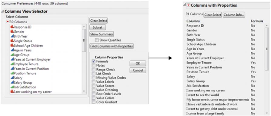
Example of Finding Columns with a Specific Property

This example shows how to find columns that have a Formula property and then view all formulas at once.

1.Open the Consumer Preferences.jmp sample data table.

2.SelectCols > Columns Viewerto open the Data Table Columns Viewer window.

3.SelectFind Columns with Properties, selectFormula, and clickOK.

The Columns with Properties report appears. Several columns include the Formula property (Figure 4.9). Because the list is so long, you want to view all formula columns together.

Figure 4.9 Select the Formula Column Property

4.Right-click the report, selectSort by Column,Formula, and then clickOK.

Columns that have a Formula property appear at the top of the report (Figure 4.10).

Figure 4.10 Sort by Column

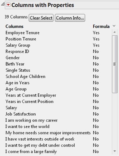
5.Select theEmployee Tenure,Position Tenure, andSalary Groupcolumns and selectColumn Info.

Formulas for the selected columns appear in the data table’s Column Settings window.

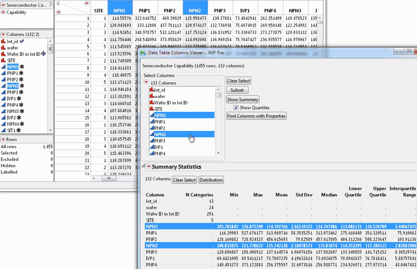
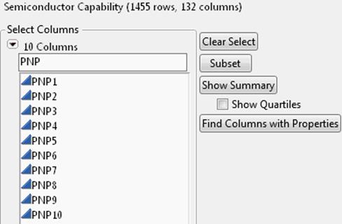
Example of Showing Summary Statistics

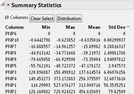
This example shows how to find columns with a low standard deviation. This can be helpful if you want to delete or exclude that data from an analysis.

1.Open the Semiconductor Capability.jmp sample data table.

2.SelectCols > Columns Viewerto open the Data Table Columns Viewer window.

3.In the Select Columns red triangle menu, selectName Starts With.

4.Type PNP and pressEnterto select thePNPcolumns (Figure 4.11).

Figure 4.11 Filter Columns by Name

5.ClickShow Summaryto add the Summary Statistics report (Figure 4.12).

The rows show the minimum, maximum, mean, and standard deviation for each column.

Figure 4.12 Summary Statistics for Selected Columns

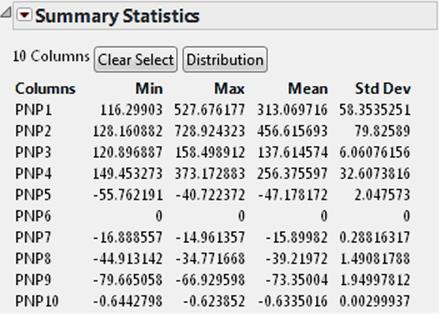
6.Right-click in the report and selectSort by Column.

7.SelectStd DevandAscending, and then clickOK.

Notice that PNP6 has no standard deviation, because the minimum, maximum, and mean values are 0.

Figure 4.13 Sorted Std Dev Column

8.In the Summary Statistics report, select the row forPNP6and then display the data table.

9.View the data table and pressDeleteto remove the selected column.

The column is instantly removed from the data table.

10.To close the Columns Viewer, click theXbutton in the upper right corner (Windows) or upper left corner (Macintosh) of the window.

Locate Next and Previously Selected Columns

You can find the next selected column after the current column by selecting Cols > Column Selection > Next Selected Column. Similarly, you can find the previously selected column before the current column by selecting Cols > Column Selection > Previous Selected Column.

Each time you select one of these options, the next or previously selected column appears and flashes. The options are available only when columns are selected.

You might want to use this feature to look at intermittently selected columns in a large data table.

Select Cells

To select a block of cells

•Drag the arrow cursor diagonally across the cells.

JMP can find all cells whose values are the same as the ones you currently have highlighted. You can do this within one data table or throughout all open data tables. Highlight the cells that contain the values that you want to locate.

To find all matching cells within the active data table

•Select Rows > Row Selection > Select Matching Cells

or

•Right-click one of the highlighted row numbers and select Select Matching Cells.

To find all matching cells across all open data tables

•Select Rows > Row Selection > Select All Matching Cells. The rows that contain the same values as the selected ones are highlighted.

To select cells that contain specific values

JMP can search for a specific value (or text string) and highlight all of the cells in the data table that contain the specific value.

1.Select Rows > Row Selection > Select Where.

Figure 4.14 Specify Criteria for Selecting Rows

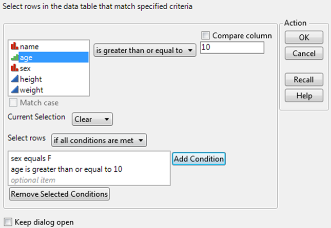
2.From the column list, highlight the name of the column whose rows you want to select.

3.Use the drop-down menu to select a condition from the list (equals, does not equal, and so on). SeeFigure 4.14.

4.Type the search value. To search for missing values, leave the box empty.

5.ClickOK.

You can also specify the following optional features:

•To compare the values of two columns, click the Compare column check box. Select from the list of columns for comparison.

•To make the search case-sensitive, click the box beside Match Case.

If you currently have rows selected in the data table, you can specify the following optional features:

•Click an option under Action on currently selected rows to tell JMP how to handle that current selection:

‒Clear Current Selection removes the highlight from currently selected rows and selects all rows that contain the specified value.

‒Extend Current Selection keeps the currently selected rows selected and also selects the rows in which the specified value has been found.

‒Select From Current Selection selects the rows in the currently selected array that contain the specified values.

•Click Add Condition to add a condition to the list.

•To add more conditions to the search, repeat the previous steps. Click the appropriate item in the Select Rows area to specify if you would like JMP to select rows conditionally: if all conditions are met, or if any of the conditions are met.

•To keep the window open after you click OK, select Keep dialog open.

Edit Data

This section describes how to edit data in a table, including editing cells and making changes to rows and columns.

Delete Rows and Columns

To delete rows

1.Highlight the rows that you want to delete.

2.Press the Delete key, or right-click on the row numbers and selectDelete Rows.

Caution: When you try to delete thousands of rows, an alert might appear if your computer has insufficient memory to save data for undo. Either select fewer rows to delete or select Disable Undo from the Table panel red triangle menu. This option removes all actions from the undo history and does not record future actions. When the Disable Undo option is selected, it is in effect only while the data table is open; the setting is not saved with the data table.

To delete columns

1.Highlight the columns to delete.

2.Press the Delete key, or right-click and selectDelete Columns.

Edit or Delete Cells

To edit or delete the contents of a cell

1.Click the cell containing the value that you want to edit or delete.

2.Press the Delete key.

3.To edit the value, click the cell a second time, and then edit the cell’s value.

Edit Column Names

To edit a column name, select the column and begin typing. You can also edit the column name in the Column Info window, or select the header and press Enter.

View Patterns of Missing Data

If your data table contains missing data, you might want to determine whether there is a pattern to the missing data. The pattern might help you make discoveries about your data.

To view patterns of missing data

1.With your data table open, select Tables > Missing Data Pattern.

2.Select the columns for which you would like to find patterns of missing data.

3.ClickAdd Columns.

4.Select theCount Missing Value Codescheck box if you want to count missing value codes as missing values.

5.ClickOK.

Example of Viewing Patterns of Missing Data

1.Open the Missing Data Pattern.jmp sample data table.

2.SelectTables > Missing Data Pattern.

Figure 4.15 The Missing Data Pattern Window

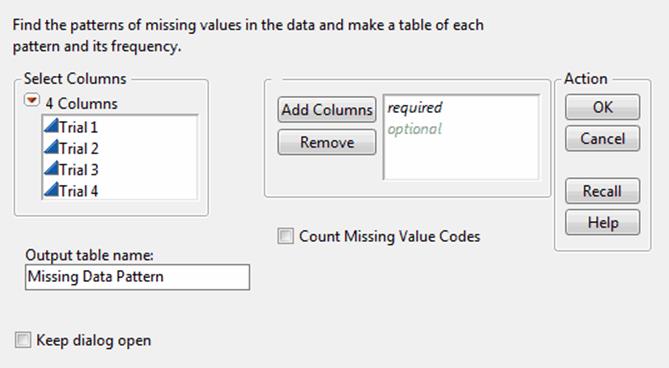
3.Highlight all of the columns.

Note: For details about the options in the red triangle menu, see “Columns Filter Menu” in the “JMP Platforms” chapter.

4.ClickAdd Columns.

5.ClickOK.

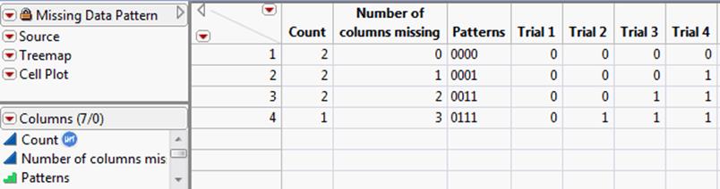
Figure 4.16 A Missing Data Pattern Table

Tip: To quickly create a Treemap or Cell Plot of the data, select Run Script from the red triangle menu next to Treemap or Cell Plot in the Table panel.

Figure 4.16 shows the following patterns:

•Row 1 shows that there are two instances where all rows in Trial 1, Trial 2, Trial 3, and Trial 4 have no missing values.

•Row 2 shows that there are two rows in the source table whose one missing value is in the Trial 4 column.

•Row 3 shows that there are two rows in the source table whose missing values are in the Trial 3 and Trial 4 columns.

•Row 4 shows that there is one row in the source table whose three missing values are in the Trial 2, Trial 3, and Trial 4 columns.

In the Missing Data Pattern table, JMP automatically assigns the Count column the analysis role of frequency. If you now use the Missing Data Pattern data table to run an analysis, JMP automatically uses Count as a frequency. So you do not have to specify Count as the role each time. For details, see “Assign a Preselected Analysis Role” in the “The Column Info Window” chapter.

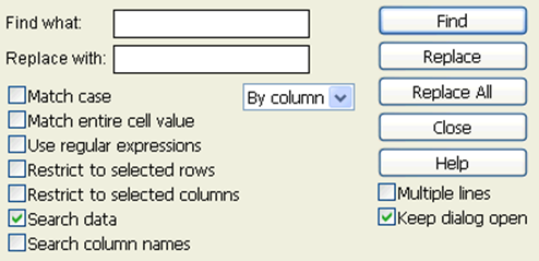
Find and Replace Cell Values

You can find and replace cell values by selecting the Edit > Search > Find options.

Figure 4.17 The Find Window

The following rules apply to searching for values:

•To find values in hidden columns, unhide the column.

•Values found in locked columns cannot be modified.

•The Undo command works only with Replace. You cannot undo Replace All.

•If your data table contains value labels, using the Search commands searches for actual values, but does not search for labels. See “Value Labels” in the “The Column Info Window” chapter.

•If your data table contains formatted values (such as dates, times, or durations) using the Search command searches for the formatted values, not the actual values.

Find Window Options

Refine your search with the following options:

Match Case

Performs a case sensitive search, which can be useful for locating proper nouns or other capitalized words.

Match entire cell value

Detects empty spaces, which lets you search for a series of words in a character column, or locate strings with unwanted leading or trailing empty spaces.

Tip: To find missing character values, leave the Find what box empty and check Match entire cell value. To find missing numeric values, insert a period into the Find box and check Match entire cell value.

Use regular expressions

Assumes the find string to be a regular expression instead of the literal string that you enter in the Find what box. The regular expressions follow standard semantics.

Restrict to selected rows

Restricts the search to selected rows.

Restrict to selected columns

Restricts the search to selected columns.

Search data

Searches only data cells (omitting column names).

Search column names

Searches only column names (omitting data cells).

By column

Searches the table column by column, from top to bottom, until it reaches the last cell in the rightmost column, or until you stop the search.

By row

Searches the data table row by row from left to right, to the rightmost cell in the last row or until you stop the search.

Multiple lines

Increases the Find and Replace boxes to 3 lines long instead of 1. The Enter key inserts a return into the field.

Tip: You can alternatively click and drag on the Find and Replace boxes to make them larger. If you copy and paste, the boxes resize to 1 line long, but all of your text is still there.

Keep dialog open

Keeps the Find window open during your search.

Search Actions

This section describes some common searches that you might perform.

Begin by searching for a value in the data table. The search begins with the first cell in the first column and searches every cell until it locates the value or reaches the end of the table.

To replace the currently highlighted cell value

Enter a value in the Replace with box and click Replace. Or, if the Search window is closed, select Edit > Search > Replace. If the replace value is a missing value, the currently highlighted cell content becomes a missing value.

To replace all occurrences of the specified value

Enter a value in the Replace with box and click Replace All. Or, if the Search window is closed, select Edit > Search > Replace All.

To replace the value and search for the next value

Enter a value in the Replace with box and click Replace. Or, if the Search window is closed, select Edit > Search > Replace and Find Next. Or, press CTRL-L.

To use a selected value as the Find what value

In the data table, select a value. Select Edit > Search > Use Selection for Find. Next, select Edit > Search > Find. The value that you selected in the data table is already entered in the Find what field.

To use a selected value as the Replace with value

In the data table, select a value. Select Edit > Search > Use Selection for Replace to populate the Replace with field.

To find the next value when the Search window is closed

Select Edit > Search > Find Next. Or, press CTRL-G, or F3 on Windows.

To find a missing value:

•To find missing character values, leave the Find what field empty and select Match entire cell value.

•To find missing numeric values, type a period into the Find what text box and select Match entire cell value.

Tip: Typing a period into the text box without clicking the Match entire cell value box searches for a period.

Reorder Columns

You can rearrange or sort data table columns by their name, data type, or modeling type, or reverse the current order. To reorder columns, select Cols > Reorder Columns and select from one of the following options:

Move Selected Columns

moves the selected columns to a particular place in the data table. Specify where to place the selected columns in the Move Selected Columns window:

‒To first: moves the selected columns so that they are in the left-most position in the data table.

‒To last: moves the selected columns so that they are in the right-most position in the data table.

‒After: moves the selected columns so that they are after a column that you identify.

Original Order

returns the columns to the order they were in when data table was last saved.

Reorder by Name

arranges the columns from left to right in alphabetical order by column name.

Reorder By Data Type

arranges the columns from left to right in alphabetic order by data type (row state, character, numeric).

Reorder By Modeling Type

arranges the columns from left to right in alphabetic order by modeling type (continuous, ordinal, nominal). Row state columns have no modeling type, and are shown last.

Reverse Order

reverses the order of the data table columns.

Group Columns

Group columns within a single heading to manage large numbers of columns and facilitate analysis role assignment. Grouped columns appear in an outline format within the Columns panel.

To group or ungroup columns

1.Within the data grid, select the columns that you want to group.

2.From the main menu, selectCols > Group ColumnsorCols > Ungroup Columns.

or

1.From the Columns panel, select the columns that you want to group.

2.Right-click on the selected columns and selectGroup ColumnsorUngroup Columns.

Note: Grouped columns are automatically retained for data tables generated from the following commands: Subset, Sort, Summary, Join, Stack, and Split. For the Stack command, if all the columns in the stack group belong to the same columns group, then the group's name is used for the column name.

Move Values

To move values in a data table, select the values, click and pause, and then drag and drop the values into the new location.

Tip: Clicking and dragging on a selection without pausing extends the selection.

When dragging and dropping values, note the following:

•Cells retain all of their characteristics and column properties.

•After you move cells, missing values appear in the cells that you initially selected.

•The selected cells and the destination cells must have the same data type.

•If you drag a set of cells to an empty area of the table, new columns are automatically created.

•New columns have the original columns’ display format and modeling types.

To specify where to move rows

1.Highlight the rows that you want to move.

2.SelectRows > Move Rows.

3.Specify where you would like to move the rows in the Move Rows window:

‒To the beginning of the table (At start)

‒To the end of the table (At end)

‒After a specific row number (After row:)

Move Content into Another Window

In Windows, you can drag selected content over a minimized window. The minimized window moves to the front and you can paste your content into it. You can do the same thing in JMP. For example, you can drag selected content over the Home Window button (located in the bottom right corner of most windows). Then in the Window List, drag the content over the window that you want to move the content into. That window moves to the front and you can drop in the content.

Tip: If you cannot see the JMP Home Window button, select View > Status Bars.

For example, you can drag a selected column, row, or cell from one data table into another; drag selected text from one script window into another; or drag selected content from a report into a journal.

Use the Row Editor

Use the Row Editor to browse or edit cells one row at a time. Open the Row Editor in one of the following ways:

•Select Rows > Row Editor.

•In a data table, double-click in the row number area. The row that you use is the row that first appears in the Row Editor.

•In a report window, right-click in a plot or graph and select Row Editor.

Figure 4.18 Row Editor

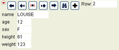
Note the following:

•If you have a report window open, and you want edited data to be automatically reflected there, make sure that Automatic Recalc is turned on. See “Automatic Recalc” in the “JMP Platforms” chapter.

•If your data table contains value labels, the Row Editor displays the label, and when the cell is highlighted for editing, it shows the actual value. See “Value Labels” in the “The Column Info Window” chapter.

Row Editor Buttons

Click the arrow buttons to browse through selected rows or the entire data set if no rows are selected. Row Editor buttons are described as follows:

Shows the previous row.

Shows the previously selected row.

Makes the row blink in graphs.

Shows the next selected row.

Shows the next row.

Searches for a row. See “Select Cells”.

Creates a new row at the end of the data table.

Note: Changes made to a row using the Row Editor are written to the data table when you change fields in the Row Editor. You still need to save the changes to the data table.

Row Editor Options

The red triangle menu in the Row Editor contains the following options:

Next Selected

displays information for the selected row that is located after the current one.

Prev Selected

displays information for the selected row that is located before the current one.

Next

displays information for the row that is located after the current one, regardless of whether the row is selected.

Prev

displays information for the row that is located before the current one, regardless of whether the row is selected.

Save

saves the data table and any changes that you have made to it via the Row Editor.

New Row

creates a new row in the data table.

Find

displays the same window as if you had selected Rows > Row Selection > Select Where. Select one of the options on the Action on currently selected rows menu, and then highlight the column whose rows you want to select. Type in the value for which you want JMP to search. See “Select Cells”.

Blink

causes the current row’s highlight to flash at a rapid rate.

Note: Text in a locked column or a locked data table cannot be edited. For details, see “Lock Tables”, and “Lock Columns in Place”.

Context Menus for Rows and Columns

When you right-click in the row number area, or at the top of a column in the column name area, context menus appear. These menus provide quick access to selected commands in the Rows and Columns menus. For details about these options, see “Context Menu for Columns” in the “Get Started” chapter and “Context Menu for Rows” in the “Get Started” chapter.

Edit Data Tables

This section describes the following actions that you can perform on data tables:

•Change the data table name

•Lock data tables

•Add table variables

•Add scripts to the data table

•Compare data tables

Change Table Names

A data table’s name appears at the top of its window, in the table panel, and on all related analysis reports. You can change a data table’s name in any of the following ways:

•Select File > Save As and save as the new name.

•In the table panel, click twice on the table name, type the new name, and then press the Enter key.

•On Windows, select Window > Set Title.

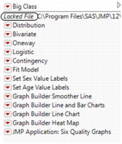
Lock Tables

Locking a JMP data table prevents data and column properties from being added or edited. You can still assign row states, run analyses, and so on. To lock a data table, click the red triangle menu next to the table name in the table panel and select Lock Data Table.

A lock icon appears next to the data table name. To unlock the file, select Lock Data Table again.

If you make a data table read-only outside of JMP (for example, by changing its properties on Windows), the data table contains a note informing you that it is locked. See Figure 4.19. This type of lock allows users to edit the data table, but not save the changes.

Figure 4.19 A Read-Only File

Compress Tables

Compressing a JMP (version 6 or higher) data table reduces the size of the stored file. You can still run analyses, assign characteristics, and so on. To compress a data table, click the red triangle menu next to the table name in the table panel and select Compress file when saved and save the data table.

After saving the data table, a compressed icon appears next to the data table name. To decompress the file, select Compress file when saved again.

In addition, you can configure JMP to always use GZ compression when saving by selecting Preferences > General > Save Data Table Columns GZ Compressed.

Note: The Compress file when saved option only decreases the file size. This command does not affect the memory required to analyze the data. To reduce both the file size and memory required for analyzing, use Cols > Compress Selected Columns. See “Compress Selected Columns”.

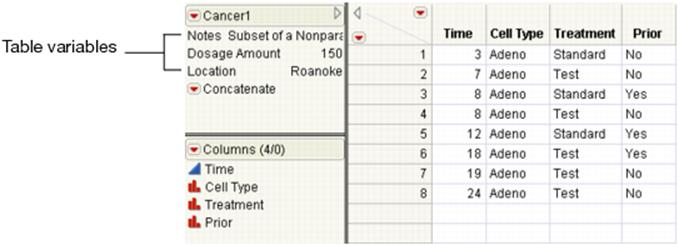
Use Table Variables

A table variable can contain textual information (for example, source information for the data), or a value that can be used by column formulas or JSL scripts. Table variable names appear in the table panel at the left of the data grid. See Figure 4.20.

Figure 4.20 Table Variables in the Table Panel

Uses for Table Variables

Use table variables in the following situations:

•To document tables

•In formulas

•In JSL scripts

Use Table Variables to Document Tables

Table variables are used primarily to document tables. Many sample data tables installed with JMP contain a table variable named Notes. This variable provides details about the data (for example, the source of the data). The example in Figure 4.20 shows a data table that contains Notes as one of its table variables. JMP also automatically creates table variables when you create a design table using the Design of Experiments commands in JMP. The design table has a table variable named Design with the name of the design type as its value.

Reference Table Variables in Formulas

Table variables can also be incorporated in formulas that you build using the Formula Editor. These formulas calculate values for a column by referring to a table variable. For details about constructing a formula that uses table variables, see “Reference Columns and Table Variables” in the “Formula Editor” chapter.

Use Table Variables in JSL Scripts

You can also incorporate table variables into JSL scripts. See the Scripting Guide for details.

Table Variable Actions

To add new table variables

1.In the Table panel, click the red triangle menu to the left of the data table name.

2.SelectNew Table Variable.

3.Give the variable a name and value in the boxes labeledNameandValue.

4.ClickOK.

The table variable appears in the Table panel.

To view or edit table variables

1.Double-click on the content of an existing table variable.

2.Edit the content.

To edit a table variable name

1.Double-click the table variable name.

2.Edit the name.

To delete table variables

Select one or more table variables and press Delete, or right-click the selected variables and select Delete. You can also press Control, right-click the blank area inside the table panel, and then select Delete Selected.

Concatenating Data Tables with Table Variables

See the “Example of Concatenating Data Tables and Table Variables” in the “Reshape Data” chapter.

Create and Save Scripts

To automatically complete various analyses and tasks, you can create a JSL script and save it to the data table. See Figure 4.21. For detailed explanations of scripts, see the Scripting Guide.

Figure 4.21 Scripts Saved With the Data Table

Save a Report Script to a Data Table

Once you have run an analysis and you are in the report window, you can add a script to the data table. This script generates the JSL that reproduces your analysis.

To save a script to the data table

•From the report window, click on the red triangle menu for the platform and select Script > Save Script to Data Table.

Example of Saving a Report Script to a Data Table

First, you create your analysis, then you save the script.

1.Open the Big Class.jmp sample data table.

2.SelectAnalyze > Fit Y by X.

3.Selectweightand clickY, Response.

4.Selectheightand clickX, Factor.

5.ClickOK.

6.From the red triangle menu for Bivariate Fit, selectFit Line.

7.From the red triangle menu, selectScript > Save Script to Data Table.

Figure 4.22 Click the Red Triangle

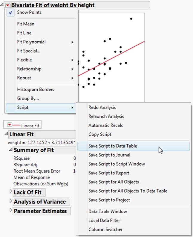
The script is added to the bottom of the Table panel.

Tip: If you want a particular script to run automatically every time the data table is opened, name the script OnOpen. Only one script saved in the data table can be set to run automatically. If you name the script Model (or model) in a Fit Model script, the launch window is automatically filled in based on the script when you select Analyze > Fit Model.

Write a JSL Script for the Data Table

To add a script to a data table using JSL

1.Click the red triangle menu to the left of the data table name in the Table panel. See Figure 4.23.

Figure 4.23 Creating a Script

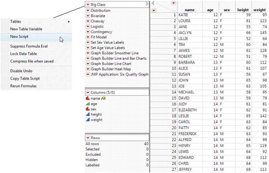
2.SelectNew Script.

3.Give the script a name by typing it into the box besideName.

4.Add the script by entering JSL code into the box besideScript.

5.Perform one of the following actions:

‒If you want to run the JSL Debugger on the script to check it for errors, click Debug Script.

‒If you are finished editing the script, click OK. The script appears in the Table panel and the window closes.

‒If you are not finished editing the script and want to save it, click Save. The script appears in the Table panel and the window remains open for further editing.

‒If you want to run the script, click Run.

Run, Edit, Delete, or Copy Scripts

To run, edit, delete, or copy a script that is saved to the data table

1.In the Table panel, click the red triangle menu beside the script’s name, or right-click on the script name.

2.Select one of the following commands:

‒Run Script

‒Edit

‒Delete

‒Copy

Once you copy a script, you can then paste it into a script window or into the Table panel of another data table.

Compare Data Tables

JMP can compare two open data tables and report the differences between data, scripts, table variables, column names, column properties, and column attributes. Character values that do not match exactly appear in the report. For numeric data, you can select a relative (or fuzzy) comparison. The numeric values are considered equal if they are within the relative error rate that you specify. The smaller the relative error, the more precise the comparison.

To compare two data tables

1.Open the data tables.

2.In one of the tables, selectTables > Compare Data Tables.

3.If necessary, select the data table that you want to compare from the list.

4.(Optional) SelectFuzzy Compareand enter the relative error to see numeric differences within the specified rate.

5.Click on the red triangle menu and select the following options:

‒which items you want to compare

‒how to show the differences

6.ClickCompare.

The Difference Summary and Difference Plot are shown by default. The red triangle options that you selected also appear.

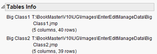
Basic Table Information

The Tables Info report shows the data table names and locations along with the numbers of columns and rows in each table. In Figure 4.24, you see that Big Class1.jmp contains one more row than Big Class2.jmp.

Figure 4.24 Basic Information

Compare Data

The interactive Difference Summary report and Different Plot indicate how rows differ between reports. Each entry in the Difference Summary report shows which action occurred, how many rows are affected, and the first row in which the change occurs.

In Figure 4.25, Big Class1.jmp (left) and Big Class2.jmp (right) are compared.

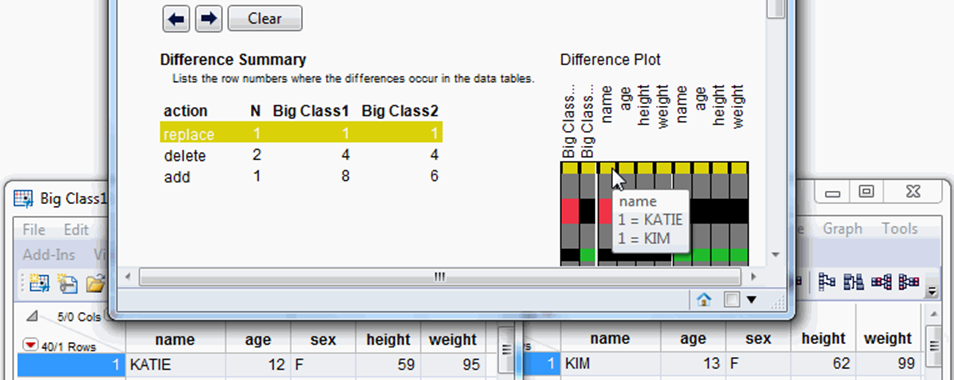
•The first entry in Figure 4.25 indicates that one row (N) has changed (or been replaced) in the first row of Big Class2.jmp. When you select the entry in the Difference Summary report on the left, the entry is highlighted in yellow, and the row flashes in the data table.

For a graphical view of the comparison, place your cursor over a colored cell in the Difference Plot. Figure 4.25 shows that the name KATIE in Big Class1.jmp was changed to KIM in Big Class2.jmp. The entire first row is highlighted in the Difference Plot, which tells you that all values in that row are different.

Figure 4.25 Modified Data

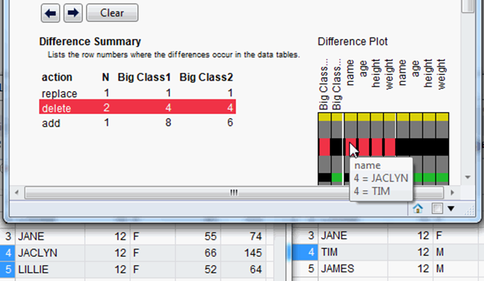
•In Figure 4.26, the second entry indicates that two rows were deleted beginning at row four. The deleted rows are highlighted in Big Class1.jmp on the left. And the Difference Plot specifies the different values. The name in row four of Big Class1.jmp was JACLYN and TIM in Big Class2.jmp.

Figure 4.26 Deleted Rows

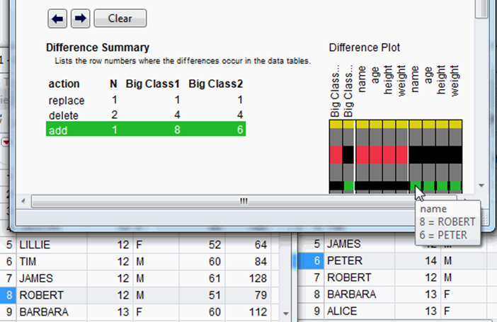
•In Figure 4.27, the third entry tells you that one row was added before what was originally row eight. The name in row eight of Big Class1.jmp was ROBERT. PETER is the name in row six of Big Class2.jmp.

Figure 4.27 Identify New Rows

Click the Previous difference and Next difference buttons above the Difference Summary to navigate from row to row.

Tip: Save the Difference Summary report to a data table by selecting Save Difference Summary from the red triangle menu.

Compare Table Properties

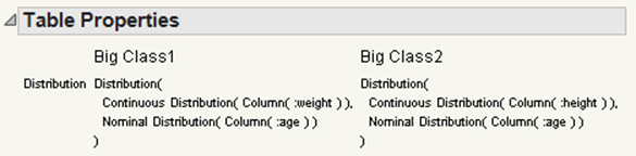
Select Compare Table Properties from the red triangle menu to see differences in table scripts and variables. For example, Figure 4.28 shows that the Distribution script in Big Class2.jmp refers to the height column rather than the weight column.

Figure 4.28 Modified Table Script

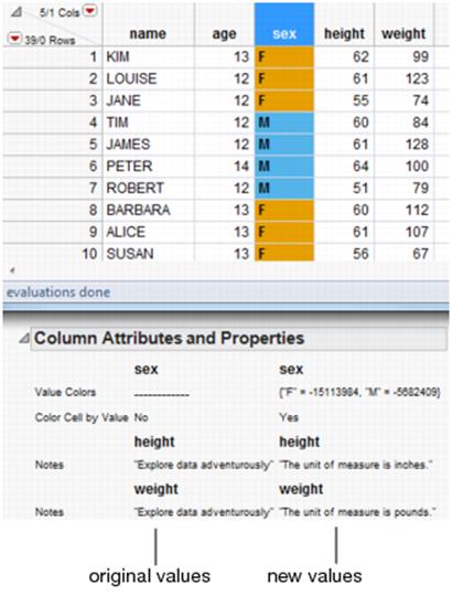
Compare Column Attributes and Properties

Select Compare Column Attributes and Properties from the red triangle menu to see differences in column notes, cell colors, and the like. For example, Figure 4.29 shows that column notes and value colors differ in Big Class2.jmp.

Figure 4.29 Modified Column Attributes and Properties

Assign Characteristics to Rows and Columns

This section describes how to exclude, hide, label, color, or mark rows and columns in order to customize the appearance of points in scatterplots and graphs. You can also lock columns so that they stay in place when you scroll through the data table.

The menu for row actions can be accessed from the following places:

•the Rows menu in the main menu

•right-click on a row

•the red triangle in the Rows panel

•the left red triangle in the upper left corner of the data grid

Similarly, the menu for columns actions can be accessed from the following places:

•the Cols menu in the main menu

•right-click on a column

•the red triangle in the Columns panel

•the right red triangle in the upper left corner of the data grid

Hide and Exclude Rows

Hiding and excluding rows means that they are hidden in plots and not analyzed.

To hide and exclude one or more rows from analyses

1.Highlight one or more rows that you want to hide and exclude.

2.Right-click on the selected rows and selectHide and Exclude.

or

From the Rows menu, select Hide and Exclude.

Exclude Rows and Columns

Marking rows and columns as excluded means that they are not analyzed. Note the following:

•Excluded observations are excluded from calculations in text reports and graphs. For most platforms, excluded observations are not hidden in plots.

•Use Hide/Unhide to hide observations in plots and graphs for most platforms. See “Hide Rows and Columns”.

•A circle with a strikethrough () appears beside either the row number or the column name in the Columns panel. The circle indicates that the row or column is excluded and therefore not analyzed.

•For most platforms, data remain excluded until you select Exclude/Unexclude again.

To exclude one or more rows from analyses

1.Highlight one or more rows that you want to exclude.

2.Right-click on the selected rows and selectExclude/Unexclude.

or

From the Rows menu, select Exclude/Unexclude.

To exclude one or more columns from analyses

1.Highlight one or more columns that you want to exclude.

2.SelectCols > Exclude/Unexcludeor right-click selectExclude/Unexclude.

To unexclude rows or columns

1.Highlight the excluded rows or columns that you want to include in your analyses.

2.SelectExclude/Unexcludefrom theRowsmenu orColsmenu. You can also right-click rows or columns and selectExclude/Unexclude.

Hide Rows and Columns

Marking rows and columns as hidden means that they do not appear in plots and graphs. Note the following:

•Hiding rows and columns does not exclude them from analyses. They simply do not appear in plots and graphs.

•To exclude hidden observations from analyses, use the Exclude/Unexclude option. See “Exclude Rows and Columns”.

•A mask icon appears beside the hidden row number or the column name, indicating that the row or column is hidden.

•Observations remain hidden until you select Hide/Unhide again.

To hide one or more rows

1.Highlight one or more rows that you want to hide.

2.Right-click on the selected rows and selectHide/Unhide

or

From the Rows menu, select Hide/Unhide.

To hide one or more columns

1.Highlight one or more columns that you want to hide.

2.SelectCols > Hide/Unhideor right-click and selectHide/Unhide.

To unhide rows or columns

1.Highlight the hidden rows or columns that you want to show in your plots and graphs.

2.SelectHide/Unhidefrom theRowsmenu orColsmenu. You can also right-click rows or columns and selectHide/Unhide.

Label Rows and Columns

When you position the arrow cursor over a point in a plot, the point’s label appears. By default, row numbers are used as labels. You can customize the labels as follows:

•You can change the label to display column values instead of the row number.

•You can enable the label to always appear, not only when you position the cursor over points.

•A label or yellow tag icon appears beside the column name in the Columns panel, indicating that points on plots are identified by the column value. If there are multiple columns that are labeled, their values appear on plots separated by a comma.

•Data remain labeled until you select Label/Unlabel again.

To change the label to display column values

1.Highlight one or more columns whose values you want to appear as the label in plots.

2.SelectCols > Label/Unlabelfrom the menu or right-click and selectLabel/Unlabel.

To enable the label to always appear (not just when you position the cursor over points)

1.Highlight one or more rows whose label you want to always appear in plots.

2.SelectRows > Label/Unlabelfrom the menu.

To turn off labeling for rows or columns

1.Highlight the labeled rows or columns that you no longer want labeled.

2.SelectLabel/Unlabelfrom theRowsmenu orColsmenu. You can also right-click columns or rows and selectLabel/Unlabel.

Assign Colors or Markers to Rows

•If you assign a color to a row, the points representing the values in that row are colored in the plot.

•If you assign a marker to a row, the point is replaced with the marker in the plot.

•You can also assign colors or markers based on column values.

Assign a Color to Rows

Assigning a color to selected rows means that the points in plots appear in the color that you select. In the data grid, the active color assigned to a row appears next to the row number.

To assign rows a color

1.Highlight one or more rows that you want to assign a color to.

2.Right-click on the highlighted rows and selectRows > Colors.

3.Select one of the available colors.

Tip: To clear an assigned color from the selected rows, assign the color black.

Add Markers to Rows

To replace the standard points in plots with a marker, use the JMP markers palette. In the data table, these markers also appear next to row numbers.

1.Highlight one or more rows that you want to apply the marker to.

2.Right-click on the selected rows and selectMarkers, and then select the marker shape.

Select Other to create custom markers. You can type alphabetic characters, numerals, and other keyboard symbols.

Tip: To return to the default marker, select the initial dot marker.

Assign Colors or Markers to Rows Based on Column Values

You can assign colors or markers to your data table rows based on the values found in a particular column. For example, in a column called Sex, you could assign all rows whose value is F a red circle marker. All rows whose value is M could have a green plus marker. These colors and markers replace the default black dot in plots and appear next to its row number in the data table.

To assign colors or markers to rows based on column values

1.Select Rows > Color or Mark by Column.

2.Select the column to color and or mark. SeeFigure 4.30.

Figure 4.30 Color or Mark by Column

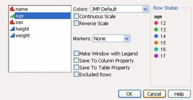
3.Select theColorsandMarkersschemes to apply.

A preview of your selection appears under Row States.

4.(Optional) Select any additional options. See“Color or Mark by Column Options”.

5.ClickOK.

6.(Optional) To shade all rows according to their row state, right-click in the row numbers area within the data grid and selectColor Rows by Row State.

From then on, the rows are shaded with the color that you assign to the rows.

Color or Mark by Column Options

Colors

select a color theme to assign different colors to the rows in your data table. Color assignment is based on the values of the selected column.

Continuous Scale

assigns colors in a chromatic sequence based on the values in the highlighted column.

Reverse Scale

assigns colors in a reversed chromatic sequence based on the values in the highlighted column.

Markers

assigns a different marker to each row in your data table based on the values found in the column that you highlighted.

Make Window with Legend

Includes a legend with your new characteristics so that you can easily identify which colors and markers correspond with which row.

Save To Column Property

saves the color and marker information as a column property. The rows in the selected column of the data table are colored, based on the color theme.

Save To Table Property

saves the color and marker information as a table property.

Excluded Rows

assigns colors or markers to rows that are excluded.

Create Color Themes

JMP includes several color themes that can distinguish a range of values in a graph. You can also create your own color themes based on an existing color theme or create custom themes.

Note: When you select a default color theme, the colors are not applied to reports that are open. You need to rerun the existing reports to format them with the default color theme.

See “Delete Custom Color Themes” for details about deleting custom color themes.

To create a color theme

1.Select File > Preferences > Graphs.

2.To either create a new Continuous Color Theme or Categorical Color Theme, click the appropriate color theme.

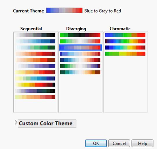
If you are creating a new continuous color theme, the Continuous Color Themes window appears.

Figure 4.31 Continuous Color Themes Window

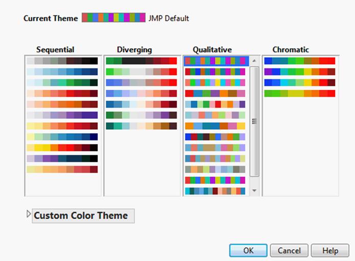
If you selected to create a new categorical color theme, the Categorical Color Themes window appears.

Figure 4.32 Categorical Color Themes Window

3.(Optional) To base the theme on an existing theme, select a color themes from the available themes.

4.Click the Custom Color Theme disclosure button to show the Custom Color Theme panel.

Figure 4.33 shows the color theme panels for both continuous and categorical themes (respectively).

Figure 4.33 Custom Color Theme Panel

5.ClickNewto create a new theme.

A new color theme is created based on the selected color theme. A temporary name is assigned to the theme.

6.Type a new name in place of the temporary label. On Windows, do not press ENTER. The window closes if you do so.

7.To modify the color theme, do any of the following:

‒To modify the gradient of continuous color, move the sliders left or right.

‒To add more colors to the gradient, click the color bar to choose a color. A new slider is displayed under the color bar.

‒To change the color of a slider, click on the slider to display the Color window and choose another color.

‒To reverse the order of the colors on the gradient, click Reverse.

‒To distribute the colors evenly on the gradient, click Space Evenly.

‒To list the custom theme in the Sequential pane, select Sequential from the drop-list.

‒To list the custom theme in the Diverging pane, select Diverging from the drop-list.

‒To list the custom theme in the Chromatic pane, select Chromatic from the drop-list.

‒To prevent a theme from appearing in lists of color themes, select Hidden.

‒To remove a color from the color theme, click the color’s slider and drag the slider above or below the color bar.

‒To discard your changes, click Cancel.

8.ClickSaveto save the custom color theme.

The new custom color theme is appended to the contents of the selected pane.

9.ClickOKto close the color theme window.

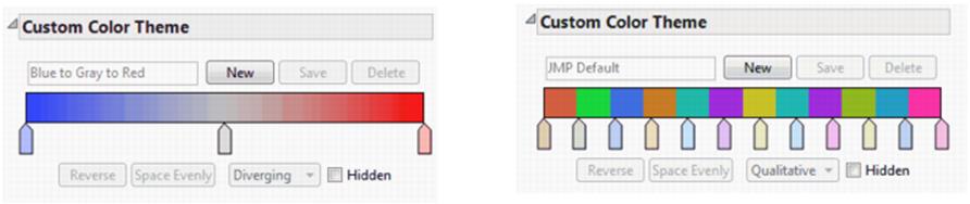
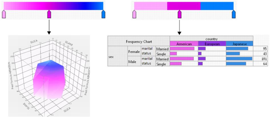
Continuous and Categorical Color Themes

The following figure shows examples of the two types of color themes in JMP, continuous and categorical. When a color theme is selected for continuous data, the colors are graduated (as shown on the left). When the same color theme is selected for categorical data, the color consists of distinct blocks of color. (as shown on the right).

Figure 4.34 Examples of Continuous and Categorical Color Themes

Custom Color Themes

Custom color themes can be applied in the same way as built-in color themes:

•You can select custom color themes as defaults from the Continuous Color Theme and Categorical Color Theme drop-down menus in the Graphs preferences. Only continuous color themes are available for continuous data. All color themes are available for categorical data.

•You can apply the custom color themes to components such as markers and data table rows. See “Assign Colors or Markers to Rows Based on Column Values” for details.

•In certain reports, such as treemaps and surface plots, you can select specific custom color themes. See the Basic Analysis book for details.

Use Custom Color Themes on Multiple Computers

In Windows, the color themes that you create are defined in the JMP preferences file called JMP.PFS. If you use JMP on more than one computer (for example, at home and at work), you can copy the color theme definitions from one JMP preferences file to another. Custom colors are then available on both computers.

In the preferences file, the code for a custom color theme looks like this:

Add Color Theme(

{"Pink to Blue", {{255, 168, 255}, {255, 0, 255}, {0, 128, 255}}}

),

In this example, the name of the color theme is “Pink to Blue.” The Red/Green/Blue (RGB) values for each color slider are located in brackets. The first slider defines the RGB values 255, 168, and 255. The second and third groups of brackets define colors for the second and third sliders.

In a text editor (such as Microsoft Notepad) add this color theme to the preferences file on your other computer. The preferences file is located in your Users folder within the JMP or JMPPro folder.

C:\Users\<user_name>\AppData\Roaming\SAS\JMP\<version_number>

C:\Users\<user_name>\AppData\Roaming\SAS\JMPPro\<version_number>

C:\Users\<user_name>\AppData\Roaming\SAS\JMPSW\<version_number>

Note: To see the preceding folders, you must configure Windows Explorer to show hidden files and folders. For details, refer to the Windows help.

To transfer color themes to another Windows computer

1.On the computer that contains the customized JMP preferences, select File > New > Script.

The Script window appears.

2.Type the following JSL function:

Show Preferences()

3.Click theRun Scriptbutton.

Your customized preferences are written to the log.

4.SelectView > Log(or display the open log).

The custom color theme that you created appears, for example:

Add Color Theme(

{"Pink to Blue", {{255, 168, 255}, {255, 0, 255}, {0, 128, 255}}}

),

This definition might be in the middle of other customized preferences that appear in the log.

5.Save the log asLog.jsland open the file on the computer whose preferences you are updating.

6.On the computer whose preferences you are updating, close JMP.

7.Make a backup ofJMP.PFS, and then open the originalJMP.PFSin a text editor.

8.Copy and paste the custom color definition fromLog.jsltoJMP.PFS. The definition goes afterPreferences(as shown in the following example:

Preferences(

Add Color Theme(

{"Pink to Blue", {{255, 168, 255}, {255, 0, 255}, {0, 128, 255}}}

),

);

Note: Be sure to include the closing parenthesis and comma. The code does not need to be indented. You can put the code in any valid location. Pasting it after Preferences( helps ensure that you do not delete any necessary parentheses or commas.

9.Save the file.

If you open JMP and the new color definition is not displayed in the preferences, delete the updated preferences file and add the definition to the original preferences file. Make sure that you copy and paste the definition in the correct location.

Delete Custom Color Themes

1.Select File > Preferences > Graphs.

2.To either delete a color theme, select either the Continuous or Categorical Color Theme.

The relevant Color Themes window appears.

3.Click the Custom Color Theme disclosure button to show the Custom Color Theme panel.

4.From the appropriate pane, select the custom color to delete.

Note: You can delete only custom color themes.

5.ClickDelete.

6.ClickOKto save your changes and close the Color Themes window.

Delete Row Characteristics

To clear all row states in the data table, select Rows > Clear Row States. To clear row states only in selected rows, select Rows > Clear Selected Row States.

All rows become included, visible, unlabeled, and show in plots as black dots. The Clear Row States command does not affect row states saved in row state columns.

Lock Columns in Place

You can lock a column in place so that when you scroll horizontally, the column remains visible. Highlight the columns and select Cols > Scroll Lock/Unlock. Note the following:

•Hidden columns cannot be scroll locked.

•The name of a locked column appears in italics in the Columns panel.

•Scroll locked columns are moved to the left in the data grid. Once you unlock them, they are not moved back to their original locations in the data table, but remain on the left.

•Columns remain scroll locked until you highlight the columns and select Scroll Lock/Unlock again.

Restructure Data

This section describes how to restructure and reformat your data. Change your data by using either the Utilities menu options, creating a new formula column, or by creating a temporary virtual column.

To restructure a column or multiple columns, select Cols > Utilities and choose from the list of options. At least one column must be selected to enable these menu options.

Make a Column into Multiple Columns

Use the Text to Columns option to make a character column with delimited fields into multiple columns. Highlight a column from a data table and select Cols > Utilities > Text to Columns. The maximum number of delimited fields across all rows determines the number of new columns created.

Note: Text to Columns is case-sensitive.

The Text to Columns window has the following options:

Delimiter

Specify text, such as a comma, to indicate how the data in the source column is organized into new columns. For example, if the original cell reads “NY, NJ, PA,” and the delimiter is a comma, three new columns are created that contain “NY”, “NJ”, and “PA”.

Make Indicator Columns

Makes new columns that are named after the distinct fields in the source column with cell values of either 0 or 1.

Include Missing

Allows any empty rows to be counted as a category. An additional column named Missing is added to the data table. A value of 1 indicates an empty row.

Make Indicator Columns

Make a categorical column into multiple columns based on each distinct category. Highlight a column in a data table and select Cols > Utilities > Make Indicator Columns. Multiple columns with values of either 0 or 1 are created. A value of 1 indicates that the original column contains that specific category.

If the given column is a Multiple Response column, the categories are determined from the set of responses.

Combine Columns

The Combine Columns option is the opposite of Text to Columns. Instead of making multiple columns, you can combine a set of columns into one character column with delimited fields.

To combine indicator columns, follow these steps:

1.Select Help > Sample Data Library and open Consumer Preferences.jmp.

2.Select the columns,Floss After Waking Up,Floss After Meal, andFloss Before Sleep.

3.SelectCols > Utilities > Combine Columns.

4.Type “Combined Floss” for the column name, and keep the default delimiter as a comma.

5.SelectSelected Columns are Indicator Columnsand clickOK.

Figure 4.35 Combined Floss Column

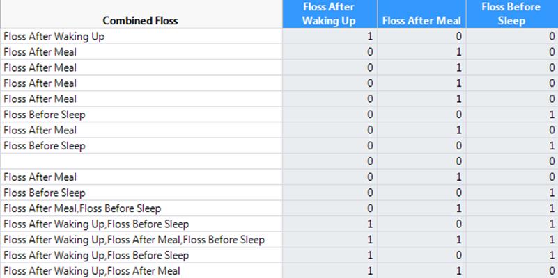
The selected columns are represented in the Combined Floss column with each field separated by a comma. Only the columns that have a value of 1 are represented in the combined column for each given row.

Compress Selected Columns

JMP lets you compress columns in a data table to minimize the size of the file and reduce the amount of memory required to analyze data. This feature is helpful when numeric columns contain many small integers or when any column contains fewer than 255 unique values. For example, compressing columns in a data table with 389 columns and 85,000 rows might decrease the file size from 250MB to 33MB, depending on the type of data.

When you compress columns, JMP verifies whether the data can be stored in a more compact form based on the data type:

•In character columns with fewer than 255 unique values, the List Check property is added to the column where appropriate (shown in Figure 4.36).

The List Check property restricts the values in the selected column to valid values. The List Check property is not applied when the number of values in the selected column is too great. For example, if the number of values is almost the same as the number of rows, the data table does not add the List Check property to the column.

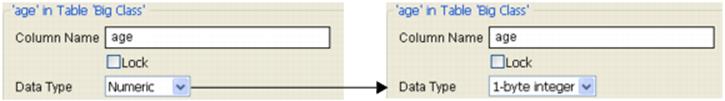
•For numeric columns, only those with the Best, Fixed Dec, or Data format are compressed. Data is compressed to 1-byte, 2-byte, or 4-byte integers when possible (shown in Figure 4.37). For details about short integers, see “The Short-Integer Format” in the “The Column Info Window” chapter.

A numeric column with non-integer values can also be compressed if there are fewer than 255 unique values. In this case, the List Check property is added to the column.

Caution: In a column with the List Check property, you can enter only a value that is in the list. Otherwise, JMP warns that the cell contains invalid data when you try to enter the new value. For details, see “List Check”.

Figure 4.36 List Check Property Added to a Compressed Character Column

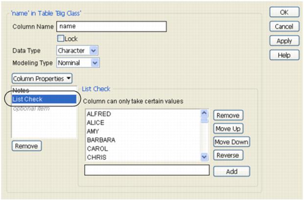
Figure 4.37 Column Info Window Showing Numeric Column before and after Compression

To compress columns, select one or more columns and select Cols > Utilities > Compress Selected Columns. (Select all columns if you do not know which columns can be compressed.)

The column or columns are compressed if possible. The log shows which columns were compressed and how they were compressed. (Select View > Log to show the log.)

Note: To compress a numeric column manually, set your Tables preferences to allow short numeric data and then change the column’s data type to 1-byte integer, 2-byte integer, or 4-byte integer. For details about this preference, see “Tables” in the “JMP Preferences” chapter.

Make Binning Formula

You can distribute your data into equal width bins using the Make Binning Formula option. Select the column or columns that you want to divide into bins, and select Cols > Utilities > Make Binning Formula. New formula columns are added to the data table.

The Make Binning Formula window contains the following options:

Format

Select a format for displaying the range of values in the bin. You can see a preview by moving the cursor over the graph.

Bin Shape: Offset

Select an offset value for the lower edge of the bins.

Note: Bins are identified by their lower edge. The lower edge is in the bin. The upper edge is in the next bin because it is the next bin's lower edge.

Bin Shape: Width

Select the width of values for the bins.

Note: The colored bands reflect the offset and the width of the bins with respect to the data.

Labels

Specify whether value labels are shown instead of the data values.

‒Select Use Value Labels to show a label instead of the value.

‒Select Use Range Values to include the lower and upper values for each range in the label.

‒Select No Labels to use the lower edge value as the label.

For more information, see “Value Labels” in the “The Column Info Window” chapter.

Tip: Value Labels are recommended in most platforms, many of which do not support range labels. In the Categorical platform, you must use value labels. On some axes, you might find that range labels more clearly identify the values.

Make All Like X

(Appears only if multiple columns are selected) Applies the choices made for the first column (X) to the remaining columns.

Make Formula Columns

Creates the formula columns and closes the window.

Example of Making a Binning Formula

1.Select Help > Sample Data Library and open Big Class.jmp.

2.Select theheightcolumn.

3.SelectCols > Utilities > Make Binning Formula.

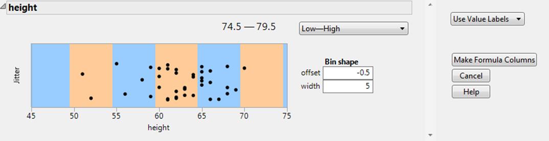
You want the range of values to appear as X-X, so keep the range set to Low - High.

4.Change theoffsetto -0.5.

Tip: For integer data, setting the offset to -0.5 helps disambiguate values on the edge. In this example, one of the bins covers 59.5 to 64.5, so it is clear that 59 and 65 are not included in this bin.

5.Keep thewidthset to 5.

6.For the labels, keep it set toUse Value Labels, so that you can see the range of values for the bin.

Figure 4.38 Completed Binning Window

7.ClickMake Formula Columns.

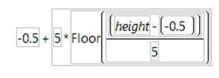
A column called height Binned is added to the Big Class.jmp data table.

8.To see how the formula is calculated, right-click on theheight Binnedcolumn and selectFormula.

Figure 4.39 Formula

Make New Formula Column

To perform further analyses on your data, use the New Formula Column menu options from your existing data table. Formula columns use formulas or calculations to define column values.

Right‐click a column heading in your data table and select New Formula Column. Choose from either Transform, Combine, Aggregate, Distributional, Date, Row, or Formula to calculate column values. A new formula column is added to the data table. See “Virtual Columns”for a description of these options.

Note: The same options exist in both the New Formula Column menu, and the right-click column menu in the launch window. However, performing these tasks in a launch window results in a temporary column, and New Formula Column adds a new column to the original data table.

Right-click options depend on the selected column’s data type and the number of columns selected. If the selected column is a Character column, Character and Row options appear. See “Character Menu” and “Row Menu” for more information.

Virtual Columns

Each launch window in JMP enables you to create one or more temporary virtual columns for use in performing analyses. These virtual columns are not part of the source data table and only can be used within the context of the current launch window. Virtual columns use formulas or calculations to define the column values. Closing the launch window or the generated report deletes any virtual columns.

Each column listed in the Select Columns pane of the launch window includes an icon representing the column’s modeling type (continuous, ordinal, or nominal) and the column name. Right-click on a column name to create a virtual column using either Transform, Combine,Aggregate, Distributional, Date, Row, or Formula to calculate the column’s values.

Right-click options depend on the selected column’s data type and number of columns selected.

Figure 4.40 Example of Virtual Column Menu

Transform

For a Numeric column, creates a virtual column based on the transcendental calculation that you select. See “Transform Menu”.

Combine

For selected Numeric columns, creates a virtual column based on the calculation that you select. See “Combine Menu”.

Aggregate

For a Numeric column, creates a virtual column based on the aggregate function that you select. See “Aggregate Menu”.

Distributional

For a Numeric column, creates a virtual column based on the distributional function that you select. See “Distributional Menu”.

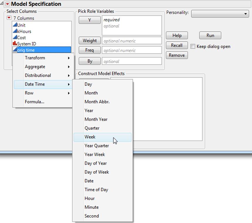
Date Time

For a column that contains date or time values, creates a virtual column based on the date/time function that you select. See “Date Time Menu”.

Row

For all data types, creates a virtual column based on the row function that you select. See “Row Menu”.

Formula

For all data types, creates a virtual column containing the custom transform data based on the formula that you select. See “Create a Formula” in the “Formula Editor” chapter for details.

Group By

For ordinal and nominal data, specifies the column to use for grouping data. A separate analysis is computed for each level of the specified column.

Note: The virtual column is available only in the current launch window. To make the virtual column available outside of the current launch window, right-click the virtual column and select Add to Data Table. The virtual column is added to the source data table.

Transform Menu

Select a function from the Transform menu to create a virtual column containing the calculations based on the selected function. For details about listed functions, see the JSL Syntax Reference. Also refer to Fitting Linear Models for additional information.

Note: You can apply unary functions to multiple columns resulting in multiple virtual columns.

The following functions are included in the menu:

Square

Calculates the square for the selected column values.

Pow10

Calculates 10 raised to the power of the selected column values.

Cube

Calculates the cube for the selected column values.

Reciprocal

Calculates the reciprocal (1/column) for the selected column values.

Negation

Calculates the negative for the selected column values.

Combine Menu

Select multiple columns to access the Combine menu. The Combine menu creates a virtual column containing the calculations based on the selected function. For details about listed functions, see the JSL Syntax Reference.

The following functions are included in the menu:

Difference

Calculates the difference between the first and second columns (A - B).

Difference (reverse order)

Calculates the difference between the second and first columns (B - A).

Ratio

Calculated the ratio of the first column to the second column (A / B).

Ratio (reverse order)

Calculates the ratio of the second column to the first column (B / A).

Average

Returns the average value of the selected columns.

Aggregate Menu

Select a function from the Aggregate menu to create a virtual column containing the statistics calculated from the selected column (or part of a column if you specified a Group By column). For details about listed functions, see the JSL Syntax Reference.

Note: The Group By option is useful for these functions.

The following functions are included in the menu:

Count

Calculates the number of values in the selected column.

Median

Calculates the median value for the selected column

Distributional Menu

Select a function from the Distributional menu to create a virtual column containing the statistics calculated from the selected column. For details about the functions listed below, see the JSL Syntax Reference.

The following functions are included in the menu:

Center

Subtracts the column mean from each value across all rows of a specified column.

Range 0 to 1

Scales the data up or down so that the minimum value is greater or equal to 0, and the maximum value is less than or equal to 1.

Box Cox

Transforms the data using the Box-Cox equation.

Johnson Normalizing

Transforms the data using one of the Johnson equations. The new column name indicates either Johnson Su, Johnson Sb, or None, depending on which equation was used to calculate the new data.

Informative Missing

Creates two columns. The Informative column replaces missing values with the column mean. The Is Missing column indicates 1 for missing values, and 0 otherwise.

Date Time Menu

For column values containing date or time values, select a function from the Date Time menu to create a virtual column containing values calculated from the selected column. For details about listed functions, see the JSL Syntax Reference.

The following functions are included in the menu:

Month Year

Returns the month number and year for the date in the selected column.

Week

Returns the number of the week in the year for the date in the selected column.

Year Quarter

Returns the year and the year’s quarter (1, 2, 3, or 4) for the date in the selected column.

Year Week

Returns a string representing the ISO-8601 week of year format (for example, June 12, 2013 results in “2013W24”).

Character Menu

Select a function from the Character menu to create a virtual column containing strings formed by the selected Character function. For details about listed functions, see the JSL Syntax Reference.

The following functions are included in the menu:

Concatenate with Space

Concatenates the strings in the selected column or columns into a new string with each sub-string separated by a whitespace.

Concatenate with Comma

Concatenates the strings in the selected column or columns into a new string with each sub-string separated by a comma character.

First Word

Extracts the first word from a character string in the selected column or columns.

Last Word

Extracts the last word from a character string in the selected column or columns.

Row Menu

Select a function from the Row menu to create a virtual column containing calculations determined by the selected Row function. For details about listed functions, see the JSL Syntax Reference.

See the Scripting Guide book for details about Row functions.

In addition to the functions described in the appendix, the following functions are included in the menu:

Difference

Calculates the difference of each value in the selected column using the formula:

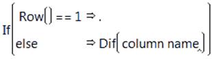
Note: The Difference function also supports the Group By option.

Cumulative Sum

Calculates the cumulative sum for each value in the selected column using the formula:

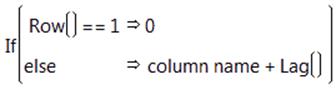
Note: The Cumulative Sum function also supports the Group By option.

Moving Average

Calculates the exponentially weighted moving average, EWMA (using a smoothing parameter between 0 to 1.0) for each value in the selected column. The following example uses a smoothing parameter of 0.25:

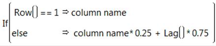
Note: JMP evaluates the formula entered on-demand therefore complex formulas might require a lot of processing time.

Virtual Column Options

After creating a virtual column, you can perform the following actions:

Rename

Renames the virtual column.

Add to Data Table

Adds the virtual column to the data table as a formula column.

Remove Transform Column

Removes the virtual column from the launch window.

Recode Data

Use the recoding tool to change all of the values in a column at once. For example, suppose you are interested in comparing the sales of computer and pharmaceutical companies. Your current company labels are Computer and Pharmaceutical. You want to change them to Technical and Drug. Going through all 32 rows of data and changing all the values would be tedious, inefficient, and error-prone, especially if you had many more rows of data. Recode is a better option.

Note: If you need to recode similar values within multiple columns, use the Recode option in Cols > Standardize Attributes. See “Standardize Attributes” in the “The Column Info Window” chapter.

1.Select Help > Sample Data Library and open Companies.jmp.

2.Select theTypecolumn by clicking once on the column heading.

3.SelectCols > Utilities > Recode.

4.In the Recode window, enter the desired values in theNew Valueboxes. For this example, enter Technical in the Computer row, and Drug in the Pharmaceutical row.

5.ClickDoneand select theIn Placeoption from the menu.

Figure 4.41 Recode Window

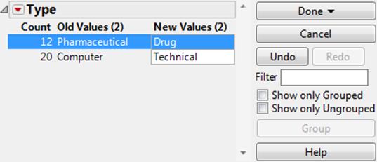
All cells are updated automatically to the new values.

Note: If you enter a non-numeric value in a column with a Numeric data type, you are prompted to convert the data type to Character. Click Yes to convert the column and display the new value. Click No to keep the column Numeric and display a missing value.

Recode Options

When you are finished recoding data, click Done to view the following options:

In Place

applies any change to the original data column.

New Column

creates a new column for the changed data and retains the original column.

Formula Column

creates a new column with the changes as a formula instead of values. Changing a value in the original column in the data table causes the formula column to update that value automatically.

Script

creates a new script called Recode in the data table. You can run this script to perform recoding in-place. If you recode additional values later, and want to update your current script, use the Script option again. You are prompted to choose if you want to merge your updates with the saved script, or create a new script. Run the Recode script immediately or after making changes to the data. You can also copy the Recode script to other data tables, or use it inside your custom scripts.

The remaining options are available on the Recode window:

Undo

reverses the last change made to the window.

Redo

recalls the last change made to the window.

Filter

searches for specific values. Add quotes around your search to find an exact phrase that includes whitespace.

Group

becomes active when multiple values are selected. Click Group to make highlighted values part of the same group. If you previously edited a value before grouping, the edited value becomes the group representative in the New Value column. Otherwise, the group representative is the value that occurs most often.

Show only Grouped

shows recoded values that have been grouped.

Show only Ungrouped

shows values that have not been grouped.

Red Triangle Options for Recode

The red triangle menu contains options for the Recode window.

Convert to Titlecase

converts the first letter of each word to uppercase, and the remaining letters to lowercase.

Convert to Uppercase

converts values to uppercase.

Convert to Lowercase

converts values to lowercase.

Tab characters, space characters, and line separators are often imported into a data table. Remove these characters using the following commands:

Trim Whitespace

removes leading and trailing whitespace characters. For example, if an extra space was imported before and after the name John, this command would delete the spaces.

Collapse Whitespace

removes leading and trailing whitespace characters and removes duplicate interior whitespace characters. That is, if more than one whitespace character is present, the Collapse Whitespace command replaces the two spaces with one space.

Use the following commands to group data based on value:

First Word

groups values based on the first word of the value. For example, if “John Smith” and “John Adams” were values, this command would group them under “John.”

Last Word

groups values based on the last word of the value.

All But First Word

groups values based on the remaining value after the first word is excluded.

All But Last Word

groups values based on the remaining value after the last word is excluded.

Group Similar Values

enables you to customize how data is grouped. Choose from the grouping options list. See “Grouping Options” below.

Start Over

returns the window to the default condition.

Recall

recalls previous changes made in the Recode window.

Script

view options to import, merge, or save Recode scripts.

‒Import From File: import a JSL script to recode previously recoded data. Run the same script on different data to recode data the same way.

‒Import From Data Table: import a JSL script saved to a data table.

‒Save to File: saves Recode changes to a JSL script. After selecting Save, you are prompted to name and save the file.

‒Save to Data Table: saves Recode script to current data table.

‒Merge with Data Table Script: merges changes made in the Recode window to the current Recode script saved to the data table. If there are multiple scripts, you are prompted to choose which script to merge your recoded data with.

‒Save to Script Window: appends the Recode script to the script window.

Right-Click Options

Right-click values in the Recode window to view the following options:

Group To

right-click selected values to select a different grouping value, or group representative. The Group To command displays the Old Values that occur most often in the data table with their corresponding New Values (if they are different). The list displays the first 8 possible group representatives.

Swap New Values

when two values are highlighted, select Swap New Values to make the new value of the first value adopt the new value of the second value, and vice versa.

Remove From Group

after values are grouped, right-click a single value or multiple values to remove them from that group.

Make Representative

right-click a single value from a group and select Make Representative to make the selected value the New Value.

Group Similar Values

right-click a single value to find values that are similar. The Grouping Options window appears. See “Grouping Options” in the section below.

Grouping Options

Select the following Group Similar Values commands to increase the accuracy of grouping:

Ignore Case

item case is ignored.

Ignore Non-Printable Characters

non-printable characters are ignored. Some data can include non-printable characters (such as file separators) that only the computer can read.

Ignore Whitespace

white space is ignored.

Ignore Punctuation

punctuation is ignored.

Allow Character Edits

allows characters to be replaced by the new value when similar values are grouped.

Difference Ratio

groups values according to proportional difference. For example, type “.25” to group values that are at least 25% different.

Max Character Difference

groups values according to a maximum number of nonadjacent character differences. For example, type “5” to group values that differ by 5 characters or less.

Example of Grouping Based on Character Difference

You can group similar values according to the number of characters that differ between them.

1.Select Help > Sample Data Library and open Candy Bars.jmp.

2.Select theNamecolumn.

3.SelectCols > Utilities > Recode.

4.From the red triangle menu, selectGroup Similar Values.

5.Select theMax Character Differenceoption and type “6”.

This allows JMP to group values that differ by a maximum of 6 characters.

6.ClickOK.

Figure 4.42 Grouped by Character Difference

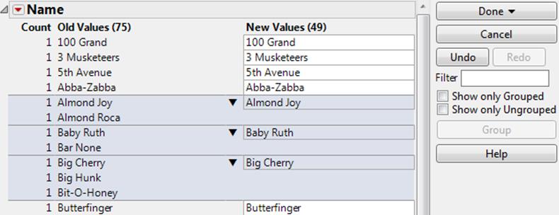
In this example, the grouped values have no more than 6 characters different between them. The values shown in the New Value column represents the grouped values in the recoded data table.

7.Right-click Almond Roca and selectMake Representativeto change the new value to represent a different value within the group.

Figure 4.43 Make Representative

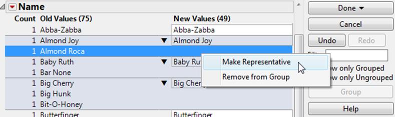
To remove values from a group, right-click and select Remove from Group.

8.ClickDone > In Placeto replace the original data with the recoded data in the table.

Example of Grouping Based on Difference Ratio

You can group similar values according to the proportion of characters that differ between them.

1.Select Help > Sample Data Library and open Candy Bars.jmp.

2.Select theNamecolumn.

3.SelectCols > Utilities > Recode.

4.From the red triangle menu, selectGroup Similar Values.

5.Select theDifference Ratiooption and type “.5”.

6.ClickOK.

This allows JMP to group values that differ by 50% or less. In other words, values that share at least 50%, or half, of the same characters. The Difference Ratio is determined by comparing the total number of characters of each value and the total amount of unique characters between two given values.

Figure 4.44 Grouped by Difference Ratio

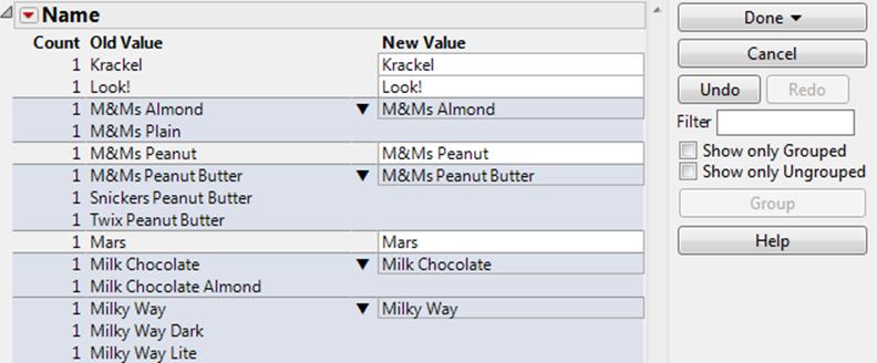
7.From the red triangle menu, selectDone > New Columnto save the recoded data in a new column in the data table.

Making a new column preserves the original data.