Using JMP 12 (2015)

Chapter 5. The Column Info Window

Set Column Attributes and Properties

Use the Column Info window to set specific properties on a column in a data table. Here are some examples of the actions that you can perform on a column:

•Change data and modeling types

•Change numeric formats

•Add formulas

•Specify restrictions on values or missing values

•Order categorical values or row data

•Save specification, control, or response limits

•Enter a known value for sigma

You can also standardize attributes and properties across multiple columns, assign a preselected analysis role to columns, and compress columns in a data table.

Figure 5.1 The Column Info Window

Contents

The Column Info Window

Column Properties

Basic Column Properties

Properties That Validate Column Values

Properties That Attach Information to Column Values

Properties That Control the Display of Columns

Properties Used in Modeling and DOE

Properties Associated with Control Charts and Capability

Properties That Control How Columns Are Used in Platforms

Additional Properties

Properties Assigned and Controlled by JMP

Standardize Attributes and Properties across Columns

Assign a Preselected Analysis Role

The Column Info Window

Use the Column Info window to specify all of the attributes and properties of a column. You can access the Column Info window in any one of the following ways:

•Select Cols > New Column

•Click an existing column heading and select Cols > Column Info

•Right-click an existing column heading and select Column Info

•Double-click directly above a column name

•In the Columns panel, right-click a column and select Column Info

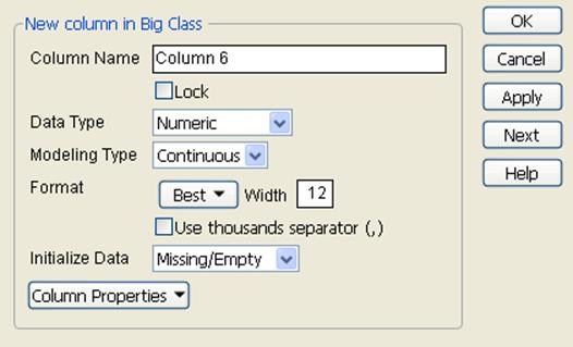
Figure 5.2 The Column Info Window

The Column Info window contains the following information:

Column Name

Type or edit the name of the column.

Lock

Lock the column so that none of its values can be edited. After you lock a column, the lock icon () appears next to the column name in the data table’s Columns panel. If you add a formula to a column, the column automatically locks.

Data Type

Select or change the data type of a column, which determines the following:

‒How the column’s values are formatted in the data grid

‒How the column’s values are saved internally

‒Whether the column’s values can be used in calculations

See “About Data Types and Modeling Types”.

Choose from the following data types:

‒Numeric columns contain only numbers (with or without a decimal point).

‒Character columns contain any characters, including numbers. In character columns, numbers are seen as characters and are treated as discrete values instead of continuous values. The maximum field width for character values is 32,766 bytes.

‒Row State columns contain row state information, which indicates whether the rows are excluded, hidden, labeled, colored, or marked. See “Row State Columns”.

‒Expression columns contain JSL expressions that can range from simple entries to complicated statement sequences. In particular, an expression can correspond to a picture, a matrix, or an expression. You can drag-and-drop expressions, such as an image, from your desktop to cells in an expression column. See “Expression Role”.

Notes:

‒If you change a column’s Data Type from Character to Numeric, any character values become missing data values and are not recoverable.

‒If you enter non-numeric data in a column with a Numeric data type, a warning window is displayed, prompting you to change the data type to Character. Click Try Again to return to the data table to re-enter the value. Click Change to change the data type. Click Revert to cancel your edit and return the cell’s value.

‒Short-integer formats might also be available. See “The Short-Integer Format”.

Modeling Type

(Numeric or Character data types only) Select or change the modeling type of a column, which tells JMP how to treat the column’s values during analyses. You can change the modeling type to look at a variable in different ways. See “About Data Types and Modeling Types”.

Choose from the following modeling types:

‒Continuous columns contain only numeric data types. Continuous values are treated as continuous measurement values. JMP uses the numeric values directly in computations.

‒Ordinal columns contain either numeric or character data types. JMP analyses treat ordinal values as discrete categorical values that have an order. If the values are numbers, the order is the numeric magnitude. If the values are character, the order is the sorting sequence.

‒Nominal columns contain either numeric or character data types. All values are treated in JMP analyses as if they are discrete values with no implicit order.

Format

(Numeric data types only) Select or change the display format of a numeric column. See “Numeric Formats”.

Initialize Data

(Appears only during new column creation) Specify the type of initial data values that you want to appear in the column. See “Fill in Initial Data Values”.

Column Properties

(Contains a list of different properties) Assign properties to columns. See “Column Properties”.

Tip: Use the Next button to continue adding columns.

About Data Types and Modeling Types

A column in a JMP data table can contain different types of information. However, all information in a single column must have the same data and modeling types.

•When you import data, JMP guesses which data and modeling types to use. Therefore, you should verify that JMP has guessed correctly.

•When you manually insert data into JMP, you should assign a data type and a modeling type at that time.

Figure 5.3 illustrates the icons that identify the different modeling types.

Figure 5.3 Modeling Type Icons in the Columns Panel

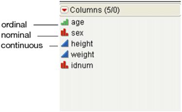
Click on an icon to change the modeling type.

Tip: You can select Continuous only if your data type is numeric. If the Continuous option is dimmed on the menu and you want to make the column continuous, you must first change the column’s data type in the Column Info window.

The Short-Integer Format

When you use the correct short-integer format for your data, you do not see any difference in how the numbers appear. However, the numbers occupy less disk space and use less memory. Short-integer formats must be activated in preferences to appear in the Column Info window.

To make short-integer formats available in the Column Info window

1.Select File > Preferences and click Tables.

2.Select theAllow short numeric data formatoption.

3.ClickOKto return to the data table.

To store numeric data in short-integer format:

1.Double-click above the column name whose values you want to be short-integer.

The Column Info window appears.

2.From theData Typemenu, select1-byte integer,2-byte integer, or4-byte integer.

JMP stores values as integers in the range that you selected. The following numbers are examples:

•For 1-byte integer, the range of numbers that you can enter is from -126 to 127.

•For 2-byte integer, the range of numbers that you can enter is from -32,766 to 32,767.

•For 4-byte integer, the range of numbers that you can enter is from -2,147,483,646 to 2,147,483,647.

Numeric Formats

For numeric columns, the Format menu appears in the Column Info window. Specify the format to tell JMP how to display numbers in the column.

Note the following information:

•For all format options, you can specify the number of total characters that you want the cells in the column to accommodate. See “Specify Width”.

•For descriptions of the format options, see “Numeric Format Options”.

•To add commas to values that equal a thousand or more, select the Use thousands separator option. You must account a space for each comma in the Width box, or else they might not appear. This option is available for the Best, Fixed Dec, Percent, and Currency formats.

Specify Width

When you specify a number in the Width field, be sure to include the total number of possible characters. Characters include: numbers, decimal points, commas, and currency symbols.

Numeric Format Options

Choose from the following numeric format options:

Best

Allows JMP to consider the precision of each cell value and select the best way to show it. By default, the physical width of the column is 12 characters.

Fixed Dec

Shows all values in the column rounded to the number of decimal places that you specify.

Note the following:

‒To see only whole numbers, set the number of decimal places to zero.

‒If the number of integers following the decimal point is smaller than the number of decimal places that you specify, zeros are added to reach the number of decimal places. For example, if the value is 1.23 and you type 5 in the Dec box, JMP shows the number with five decimal places: 1.23000.

Percent

Multiplies numeric values by 100 and shows the number followed by a percent sign.

PValue

Shows probability values. The default value of the width is 12. If a number is less than 0.0001, the number is displayed as <.0001. The format is mostly used in JSL scripts and rarely needed for a data table column.

Scientific

Shows a number in standard scientific notation. If you enter the number 123456, it appears as 1.23456e+5. Select Dec to show the decimal points and enter the number of points.

Engineering

Similar to Scientific, but the exponent is always a multiple of 3 and the Dec field represents significant digits.

Engineering SI

Same as Engineering, but the exponent is replaced with an SI symbol.

Precision

Rounds the number to a given number of significant digits.

Currency

Formats values with two decimal positions, thousands separators, and the currency sign that is specified in your computer’s locale settings. The default width of the Currency format is 15. If you have a number that requires a wider field width, the format defaults to the Best format. Once assigned, the currency symbol appears in the column and in graphs that contain the column.

Date

Shows all values in the column as a date. See “Date Formats”.

Time

Shows all values in the column as a specific instance in time, such as 12/2/03 at 2:23 PM. See “Time Formats”.

Duration

Shows all values in the column as a duration of time, such as hours, minutes, and seconds.

‒:day:hr:m, :day:hr:m:s show a duration of time, such as 52:03:01:30, or fifty-two days, three hours, one minute, and thirty seconds.

‒hr:m, hr:m:s, min:s shows a duration of time, such as 17:37, or seventeen hours and thirty-seven minutes.

Geographic

Shows latitude and longitude number formatting for geographic maps. Latitude and longitude options include the following:

‒DDD (degrees)

‒DMM (degrees and minutes)

‒DMS (degrees, minutes, and seconds)

In each format, the last field can have a fraction part. You can specify the direction with either a signed degree field or a direction suffix. To show a signed degree field, such as -59°00'00", deselect Direction Indicator. To show the direction suffix, such as 59°00'00" S, select Direction Indicator.

To use spaces as field separators, deselect Field Punctuation. To use degrees, minutes, and seconds symbols, select Field Punctuation.

Date Formats

When you choose a Date format, you can also specify an Input Format. The Date format indicates how the date appears in the data table cells, and the Input Format indicates how you enter the date.

If you assign a date format to a numeric column that already contains data, then the numeric values are treated as the number of seconds since January 1, 1904. For example, if you have a numeric column with a cell value of 1,234,567,890 and you change the format to Date > m/d/y, the cell value appears as 02/13/1943.

The examples in Table 5.1 use the date of December 31, 2004.

Note: To change how a date appears in a graph without changing how it appears in a data table, see “Change the Numeric Format of an Axis” in the “JMP Platforms” chapter.

Time Formats

When you choose a Time format, you can also specify an Input Format. The Time format indicates how the time appears in the data table cells, and the Input Format indicates how you enter the time.

•You can add the number of hours, minutes, and seconds after midnight of the prepended date for the following date formats:

‒m/d/y

‒d/m/y

‒y/m/d

‒ddMonyyyy

‒Monddyyyy

‒Locale Date

For example, December 31, 2004 has a numeric value of 3,187,296,600, which represents 12/31/2004 12:10 AM.

•:day:hr:m and :day:hr:m:s show the number of days, hours, minutes, and seconds since January 1, 1904. For example, the results for December 31, 2004 are :36890:00:10: and :36890:00:10:00.

•h:m:s and h:m show the hours, minutes, and seconds portion of the date in the date field. For example, the results for December 31, 2004 at 12:10 AM are 12:10:00 AM and 12:10 AM.

•yyyy-mm-ddThh:mm and yyyy-mm-ddThh:mm:ss show the year, month, day, and time. For example, 2004-12-31T12:10:00. T is a literal value, representing itself.

Note: To change how a time appears in a graph without changing how it appears in a data table, see “Change the Numeric Format of an Axis” in the “JMP Platforms” chapter.

International Formats

If you are importing or entering data that contains formatting specific to country standards, you might need to make sure that your number formats are interpreted correctly. On Windows, access the Control Panel’s region and language option, and select the country for which the number should be formatted. On the Macintosh, from the Apple menu, select System Preferences > Language & Text> Formats, and select the correct country. On later versions of Macintosh, this option may appear under System Preferences > Language and Region.

Row State Columns

Similar to assigning row states to rows, you can create a column that contains only row state information. A row state column stores information about whether rows are excluded, hidden, labeled, colored, marked, or selected. To designate a column as a row state column, in the Column Info window next to Data Type, select Row State.

Figure 5.4 Row States in Rows and a Row State Column

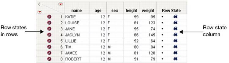
Since row state columns store the row states, you can apply them again later. Populate row state columns by copying them from the current row states or with column formulas.

To create a row state column

1.Select Cols > New Column.

2.Next toData Type, selectRow State.

3.ClickOK.

Populate the cells with new row state information or copy existing row state information from rows.

To populate cells with new row state information

1.To populate only certain rows in the row state column, highlight those rows. Or, to populate all rows in the column, highlight the row state column.

2.Right-click and selectRow States Cells.

3.Select the row state that you want to apply.

To copy existing row state information

1.To populate only certain rows in the row state column, highlight those rows. Or, to populate all rows in the column, highlight the row state column.

2.Click the star icon beside the column name in the Columns panel.

3.Select one of the following:

‒Copy from Row States Replaces the row states in the column with the row states from the rows.

‒Add from Row States Adds the row states from the rows to the row state column.

‒Copy to Row States  Replaces the row states in the rows with the row states from the column.

‒Add to Row States Adds the row states from the row state column to the row states in the rows.

Permanently Select Cells

You can save a selection in a row state column just like you save other row state characteristics (hide, exclude, color, and so on). This places a “permanent” highlight on a cell.

To permanently select cells

1.Right-click a cell and select Row States Cells > Select/Deselect.

2.Repeat this for as many cells as you would like to select.

3.To remove the highlight, right-click on the cell and selectRow States Cells > Select/Deselect.

Fill in Initial Data Values

When you add a new column to a data table, the Initialize Data menu appears in the Column Info window. Specify the type of initial data values that you want to appear in the new column. Select one of the following options:

Missing/Empty

Places missing values in the column, represented by a black dot (•) for numeric data and a blank space for character data.

Constant

Places one number or character in all of the column’s rows. Enter the number or character into the box that appears. Enter any number of characters.

Today

Places today’s timestamp in the column for each row. This option is relevant only for the Date or Time formats.

Sequence Data

Inserts sequential data based on the parameters that you specify. See “Numeric or Character Sequence Data”.

Random

Inserts random data into the column. Select the type of random number that you want to use, and then enter one of the following:

‒A range for random integers or random uniform numbers.

‒The mean and standard deviation for random normal numbers.

‒Values and proportions for random indicators.

Numeric or Character Sequence Data

To insert sequential data for numeric data

1.Next to Data Type, make sure Numeric is selected.

2.Next toInitialize Data, selectSequence Data.

3.In theFromandToboxes, assign a starting and ending point.

4.In theStepbox, assign the sequence.

5.(Optional) In theRepeat each value N timesbox, enter the number of times that you want each numeric value repeated.

6.ClickOK.

For example, if you want the column to contain even numbers from 2 to 60, type 2 in the From box, 60 in the To box, and 2 in the Step box.

To insert sequential data for character data

1.Next to Data Type, make sure Character is selected.

2.Next toInitialize Data, selectSequence Data.

3.In the box next toAdd, enter the character data and clickAdd.

4.(Optional) In theRepeat each value N timesbox, enter the number of times that you want each character value repeated.

5.ClickOK.

Column Properties

A column property is information that is attached to a column. Once that information is entered, it is saved as part of the data table. You can select column properties and apply them to columns. There are some column properties that JMP creates for your convenience. Often, you can modify these.

Column properties are listed in the Column Info window’s Column Properties menu. The area below the Column Properties menu shows column properties that have been saved to a column. To view or edit a property, select it from this list.

In the Columns panel of the data table, an icon appears next to the name of each column that contains a property, other than the Notes property. The Notes property is not denoted by an icon. Icons include the following:

Indicates that the range or list check property is applied

Indicates that the column contains a formula

Indicates that the column contains a property other than the Note, Range Check, or List Check column property

To assign a column property to one or more columns

1.Select the column or columns to which you want to assign a property.

2.Do one of the following:

‒Right-click the header area, select Column Properties, and select the property.

‒Right-click the header area, select Column Info, and select the property from the Column Properties menu.

‒Select Cols > Column Info and select the property from the Column Properties menu.

3.In the column property panel that appears, specify values and select options as appropriate.

•Click Apply to add the column property or click OK to add the column property and close the column properties window.

A column might already contain a property that you want to apply to other columns. Use the Standardize Attributes command to apply that property to other columns. See “Standardize Attributes and Properties across Columns”.

The following sections describe the properties that you can add to columns.

Basic Column Properties

Basic column properties that apply generally include Formula and Notes.

Formula

Insert a formula into a column to compute the values for that column. After a formula is added, the column is locked so that its data values cannot be manually edited (preventing invalidation of the formula).

•Click Edit Formula to create a formula. For details about creating a formula, see the “Formula Editor” chapter.

•If you do not want JMP to evaluate the formula, click Suppress Eval.

•If you do not want JMP to alert you about errors in your formula, click Ignore Errors.

•Once you have created a formula:

‒In the Column Info window, a visual of the formula appears at right. However, if your formula is long, only a portion of it might appear. Click and drag the borders of the formula box to resize it.

‒From the data table, edit the formula by clicking () next to the column name in the Columns panel.

Tip: To bypass the Column Info window when creating a formula, right-click on the column and select Formula.

Notes

Adds notes to the selected column.

Properties That Validate Column Values

The following properties help validate values in a column: Range Check, List Check, and Missing Value Codes.

Range Check

Range checking validates the data in a column. Set up the column to accept only numbers that fall within a specified range.

Select which formula to use to set up the range. x is the value entered into the column, a is the beginning of the range, and b is the end of the range.

a = the lowest value that the column accepts

b = the highest value that the column accepts

For a single-sided range check, leave either a or b empty.

From the data table, modify the range check by clicking () next to the column name in the Columns panel.

To turn off range checking

1.From the data table, right-click the column name in the Columns panel.

2.SelectValidation > No Checking.

List Check

List checking validates the data in a column. Set up the column to accept only the individual values that you specify. List checking is useful when you want to specify how to order the data in your graphs or plots.

Use the buttons to add new values, change, or reverse the order of values, and remove values.

Once a list check is set on a column, the cursor changes to when positioned over the cells. If you try to enter a value not included on the validation list, a warning message appears.

To see a menu of acceptable values, right-click a cell and select List Check Values. You can select the cell value from the menu instead of entering it into the cell.

From the data table, modify the list check by clicking next to the column name in the Columns panel.

To turn off list checking

1.From the data table, right-click the column name in the Columns panel.

2.SelectValidation > No Checking.

Missing Value Codes

Use missing value codes to specify column values that should be treated as missing. For example, sometimes the value 99 is used as a placeholder to represent missing values, or perhaps several values are used to represent different types of missing values.

Note: The Missing Value Codes column property is an extended attribute. If you plan to export to a SAS 9.4 server or Save As a SAS 9.4 file format, you should enable extended attributes in the SAS Integration Preference page. See “SAS Integration” in the “JMP Preferences” chapter for details. Alternatively, you should select Store table and column properties in SAS 9.4 extended attributes in the Save As window. If extended attributes are not selected, JMP exports or saves Missing Value Codes as missing values. Extended attributes are supported only by SAS 9.4. Earlier versions of SAS disregard any extended attributes.

Properties That Attach Information to Column Values

The following column properties attach information that is used in reports and plots to the values in a column:

•Value Labels

•Value Scores

•Value Ordering

•Row Order Levels

•Value Colors

•Color Gradient

Value Labels

Use value labels to show a label in the data table instead of a value. A label appears for each instance of the value. You can show the original values by double-clicking a label within a cell.

•Enter the value that you want to assign a label to in the Value box.

•Enter the label that you want to appear in the Label box.

•To use ranges, click Allow Ranges then specify the lower and upper values.

Note: If Allow Ranges is selected, Value Labels can be non-integers. Graph Builder can use the Value Labels for the x- and y-axes.

Tip: To assign a label to missing values, enter a period (.) for the lower bound and leave the upper bound empty. To assign a label to all other values, enter three periods (...) for the lower bound and leave the upper bound empty.

•Add, change, or remove labels.

Note the following tips:

•To turn off value labels in the data table without deleting the value labels that you have set up, in the Column Properties window, deselect Use Value Labels. Or, to quickly show or hide value labels in a data table, right-click on a column and check or uncheck Use Value Labels.

•When your data table contains value labels, using the Search commands searches for actual values, but does not search for labels.

•When your data table contains value labels, the Row Editor displays the label, and when the cell is highlighted for editing, it shows the actual value.

•If you copy and paste a cell with a value label, the actual value is pasted.

•In a formula, when you reference a column using value labels, hold your mouse pointer over the value label to see the actual data value.

Value Scores

Use value scores to indicate a value-score pair for categorical data columns. The value is a data value and the score is a number. This property associates a data value with a score (for example, the column’s data value could be “not satisfied”, “satisfied”, “very satisfied”). The user could assign a score of 0 to “not satisfied”, 50 to “satisfied”, and 100 to “very satisfied”. Those scores are then used for computation purposes like computing the mean. See the Categorical chapter in Consumer Research for an example.

To use Value Scores:

1.In the data table, right-click on the column and select Column Info.

2.From theColumn Propertieslist, selectValue Scores.

3.Enter the value that you want to assign a label to in theValuebox (for example, “satisfied”).

4.Enter the label that you want to appear in theScorebox (for example, “50”).

5.ClickAdd,Change, orRemove.

6.ClickOK.

Value Ordering

Value Ordering assigns an ordering to values in a column that is then used in reports and plots. The default ordering for reports and plots is alphanumeric data value ordering.

When you construct a design using a DOE platform, the Value Ordering column property is automatically assigned to categorical factors. For examples of assigning and editing the Value Ordering column property, see the Design of Experiments Guide.

Note: If you use both the Value Ordering and Row Order Levels properties, the Value Ordering property overrides the Row Order Levels.

The following values automatically appear in the appropriate order in reports:

•January, February, March, April, May, June, July, August, September, October, November, December

•Jan, Feb, Mar, Apr, May, Jun, Jul, Aug, Sep, Oct, Nov, Dec

•Sunday, Monday, Tuesday, Wednesday, Thursday, Friday, Saturday

•Very Low, Low, Medium Low, Medium, Medium High, High, Very High

•Strongly Disagree, Disagree, Neutral, Indifferent, Agree, Strongly Agree

•Failing, Unacceptable, Very Poor, Poor, Bad, Acceptable, Average, Good, Better, Very Good, Excellent, Best

Tip: You can anonymize Value Ordering so that the Value Ordering properties are renumbered. To do this, highlight the column with the Value Ordering column property and select Tables > Anonymize.

Row Order Levels

Use the Row Order Levels property to sort the column values by their occurrence in the data, rather than sort by value.

The row ordering applies only to the selected column. To apply it to other columns, repeat the above steps for each column, or use the Standardize Attributes command. See “Standardize Attributes and Properties across Columns”.

Tip: To show the analyzed row data in another order (besides according to their values or their occurrence in the data table columns) use the Value Ordering property. See “Value Ordering”. The Value Ordering property overrides the Row Order Levels property when both are evoked.

Value Colors

Use value colors to assign the values of a nominal or ordinal column a certain color or range of color themes. The column’s values appear with the assigned color in all applicable graphs, such as mosaic plots and plots with color-coded legends. You can also color the values in the data table column.

•To change the color of a specific value, right-click a color circle and select a color.

•To use a color theme, select it from the Color Theme menu.

•To create a custom color theme, see “Create a Custom Color Theme”.

•To also color the cells in the data table, select Color Cell by Value.

•(Optional) Select from the options in the Macros menu. See “Macros Options”.

Create a Custom Color Theme

To create a custom color theme

1.Select Custom from the Color Theme menu.

2.Create the color using the sliders.

3.Name the color and clickSave.

4.ClickOKtwo times.

You can access the new custom color in the Color Theme menu the next time you use the Value Colors property. The color is also saved in your preferences. See “Create Color Themes” in the “Enter and Edit Data” chapter.

Macros Options

The Macros menu contains the following options:

Gradient between ends

Sets the colors of the top and bottom values. JMP applies a color gradient across the entire range of values. Use this command to make all of the colors in between for the other levels.

Gradient between selected points

Sets the colors of the top and bottom values so that JMP can apply a color gradient to a range of values that you have highlighted in the Value Colors list.

Reverse colors

Reverses the color of the values from top to bottom or bottom to top.

Revert to old colors

Sets the colors back to their original color values.

Color Gradient

Select a color gradient to color a continuous column in a plot. Color gradients are supported in the Graph Builder, Bubble Plot, Treemap, and Cell Plot platforms.

•To also color the cells in the data table, select Color Cell by Value.

•Select a color gradient from the menu.

•Enter the minimum, maximum, and center values:

‒Minimum values reflect the color at the left of the gradient.

‒Maximum values reflect the color at the right of the gradient.

‒Center values reflect the color in the middle of the gradient.

Note: To see color gradients in Graph Builder, you must assign the column to the Color zone. To see color gradients in Bubble Plot and Treemap, you must assign the column to the Coloring role.

Properties That Control the Display of Columns

The Axis and Units column properties control how column values are displayed.

Axis

Use the Axis property to change the default axis settings for a column. JMP automatically uses your settings when the column appears in an analysis.

Specify the following properties in the Axis panel:

Scale Type

Change the scale type to Linear, Log, Geodesic, or Geodesic US.

Min

Set the minimum value in the graph.

Max

Set the maximum value in the graph.

Minor Ticks

Specify the number of minor tick marks in the graph.

Inc

Specify the number of increments in the graph.

Show Major Ticks

Show major tick marks in the graph.

Show Minor Ticks

Show minor tick marks in the graph.

Show Major Grid

Show major gridlines in the graph.

Show Minor Grid

Show minor gridlines in the graph.

Inside Ticks

Show axis tick marks inside the graph frame.

Show Labels

Show labels in the graph.

Orientation menu

Change the orientation of the axis labels. Choose from the following options:

‒Automatic adjusts the orientation based on the length of the label text.

‒Horizontal and Vertical describe orientations for single axes.

‒Perpendicular and Parallel describe orientations for paired axes (for example, in Scatterplot Matrices).

‒Angled adjusts the orientation to be angled at a 45 degree angle.

To set default axis properties for a column from within a graph

1.Create the graph.

2.Change the axis to your preferred specifications. See“Customize Axes and Axis Labels in the Axis Settings Window”in the “JMP Platforms” chapter.

3.Right-click the axis and selectSave to Column Property.

Units

Use the Units property to specify the measurement units that were used to collect the data for the column. The units appear in parentheses after the column name in the data table and when the column appears in plots. For example, you might want a column to indicate that age values are measured in months, or that a monetary value is in thousands of dollars.

Properties Used in Modeling and DOE

When you construct a design using the DOE platforms, column properties are saved to the resulting design table. However, some of these column properties are useful in general modeling situations. To use the properties more generally, you can specify them yourself.

Note: The Design of Experiments Guide describes the properties associated with DOE in detail and presents examples. Only a brief description of these properties is provided here.

The following column properties are used in modeling and DOE:

•Response Limits

•Design Role

•Coding

•Mixture

•Factor Changes

Response Limits

The Response Limits column property defines a desirability function for the response. The Prediction and Contour Profilers use desirability functions to find optimal settings. For more information, see the Design of Experiments Guide.

Design Role

The Design Role column property indicates how a column is used in both a designed experiment and in the model used to fit the data. For example, a column could represent a continuous factor, a categorical factor, a blocking factor, and so on. For more information, see the Design of Experiments Guide.

Coding

The Coding column property applies a linear transformation to the data in a numeric column. The data are transformed to –1 and +1 based on bounds that you specify. JMP then uses the transformed data values whenever the column is entered as a model effect in the Fit Model platform. For more information, see the Design of Experiments Guide.

Mixture

The Mixture column property is useful when a column in a data table represents a component of a mixture. The components of a mixture are constrained to sum to a constant. The Mixture column property identifies a column as a mixture component and defines a coding for that column. For more information, see the Design of Experiments Guide.

Factor Changes

The Factor Changes column property indicates how difficult it is to change factor settings in a designed experiment. It is used to create and analyze split-plot, split-split-plot, and two-way split-plot designs. For more information, see the Design of Experiments Guide.

Properties Associated with Control Charts and Capability

The Specification Limits, Control Limits, and Sigma properties are associated with control charts and capability.

Spec Limits

Specification limits are used when you perform a capability analysis using the Distribution and Capability platforms.

You can specify any combination of a Lower Spec Limit, an Upper Spec Limit, or a Target. The Show as graph reference lines option displays the specification limits and target that you specify as reference lines on appropriate plots.

Control Limits

The Control Limits column property enables you to specify control limits for a column, rather that having JMP calculate control limits from the values in the column. This is useful when you are comparing process data to historical control limits.

The Control Limits column property can be assigned only to a numeric column. To assign the Control Limits column property, select the control chart type and then enter the requested values. If any of these entries are missing, JMP replaces it with a calculated value in the control chart.

Sigma

Use the Sigma property to enter a known sigma value. This value is used by applications such as control charts or any application that requires a sigma value to complete computations. If no sigma value is supplied, sigma is calculated from the sample.

Properties That Control How Columns Are Used in Platforms

The following properties control how columns are used in platforms:

•Distribution

•Time Frequency

•Map Role

•Supercategories

•Multiple Response

•Profit Matrix

•Informative Missing

Distribution

For a column that contains continuous numeric data, use the Distribution property to select a distribution type to fit to the column. When you run the Distribution report (Analyze > Distribution) for the column, JMP automatically estimates a fit using the specified distribution. A curve reflects when the data completely fits the specified distribution.

Set the Distribution property only when you already know how the data is distributed. For example, you might already know before you run Analyze > Distribution that the data has a Weibull distribution.

If you set the Distribution property and the Spec Limits property, then the Distribution report produces a Capability Analysis report, reflecting the distribution type that you selected for the column.

Time Frequency

When using the Time Series platform, you can assign the Time Frequency property to data. The Time Frequency property specifies the frequency with which the data is reported (such as annually, quarterly, monthly, and so on). Specifying a time frequency allows JMP to take things like leap years and leap days into account. If no frequency is specified, the data is treated as equally spaced numeric data.

Map Role

If you have created a data table that contains boundary data (such as countries, states, provinces, or counties), to see a corresponding map in Graph Builder, use the Map Role property.

Note the following:

•If the custom boundary files reside in the default custom maps directory, then you need to specify only the Map Role property in the -Name file.

•If the custom boundary files reside in an alternate location, then you must specify the Map Role property in the -Name file and in the data table that you are analyzing.

•The columns that contain the Map Role property must contain the same boundary names, but the column names can be different.

Note: For an example using the Map Role property, see Essential Graphing.

To add the Map Role property into the -Name data table

1.Right-click on the column containing the boundaries and select Column Properties > Map Role.

2.SelectShape Name Definition.

3.ClickOK.

4.Save the data table.

To add the Map Role property into the data table that you are analyzing

Note: Perform these steps only if your custom boundary files do not reside in the default custom maps directory.

1.Right-click on the column containing the boundaries and select Column Properties > Map Role.

2.SelectShape Name Use.

3.Next toMap name data table, enter the relative, or absolute path to the-Namemap data table.

If the map data table is in the same folder, enter only the filename. Quotation marks are not required when the path contains spaces.

4.Next toShape definition column, enter the name of the column in the map data table whose values match those in the selected column.

5.ClickOK.

6.Save the data table.

When you generate a graph in Graph Builder and assign the modified column to the Shape zone, your boundaries appear on the graph.

Supercategories

When a data set contains ratings (for example, on a five-point scale), you might want to know the percent of the responses in a subset of those ratings. Add a Supercategories column property to group specific categories into one category.

Supercategories are supported only in the Categorical platform.

To add the Supercategory property to a data column

1.Right-click the column that contains categories that you want to group.

2.SelectColumn Properties > Supercategories.

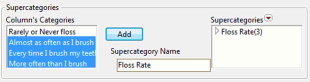
The column properties window shows the Supercategories options (Figure 5.5).

3.Select the categories in the Column’s Categories list that you want to group.

4.Enter a descriptive name next to Supercategory Name.

Leave the name blank, and JMP names the supercategory after the categories that you selected.

5.ClickAddto create the supercategory.

6.From theSupercategoriesred triangle menu, select from the following options:

‒Options > Hide: Hides data in the selected supercategory from reports and graphs.

‒Add All: Creates a supercategory from all of the categories in the column.

‒Add Mean and Add Std Dev: Calculate statistics for value scores. See the Consumer Research book for more information.

7.ClickOKto add the property to the column.

Figure 5.5 Example Supercategories Configuration

Multiple Response

Some column's data values might have more than one response in each data cell. For example, a cell in the Brush Delimited column in the Consumer Preferences.jmp sample data table contains the values “Wake, After Meal, Before Sleep”. For a column that contains multiple responses, use the Multiple Response property to configure the Separator character used to separate the responses within a data cell.

Figure 5.6 Example Multiple Response Configuration

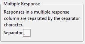
Note: You can use the Multiple Response property in the Categorical platform. See the Consumer Research book for details. You can also use this property in the Data Filter. See the Platforms chapter in the Using JMP book.

Profit Matrix

Use the Profit Matrix property to enhance a predictive model by converting it to a decision model and assigning weights to outcomes. To access the feature, select Column Properties > Profit Matrix. A matrix table appears, using each value in the selected column.

•Enter positive numbers as projected profits for correct decisions.

•Enter negative numbers as projected costs for incorrect decisions.

Each row shows the consequences if you predicted this response. Each column shows the consequences if the actual response if this response. The Undecided row indicates any associated profits or costs for situations where no decision is made. For example, an airline can charge a penalty in addition to the reservation fee for purchasing a ticket within 48 hours of the scheduled departure. Alternatively, if an airline has a lot of openings on a scheduled flight the day before the departure, they might offer a bonus as an incentive to selling tickets.

After completing the profit matrix, save the prediction formulas for use in creating best decision columns. The best decision is the one with the greatest expected profit. The example below (Figure 5.7) uses the Airline column in the Travel Costs.jmp sample data table.

Figure 5.7 Example of Profit Matrix Window

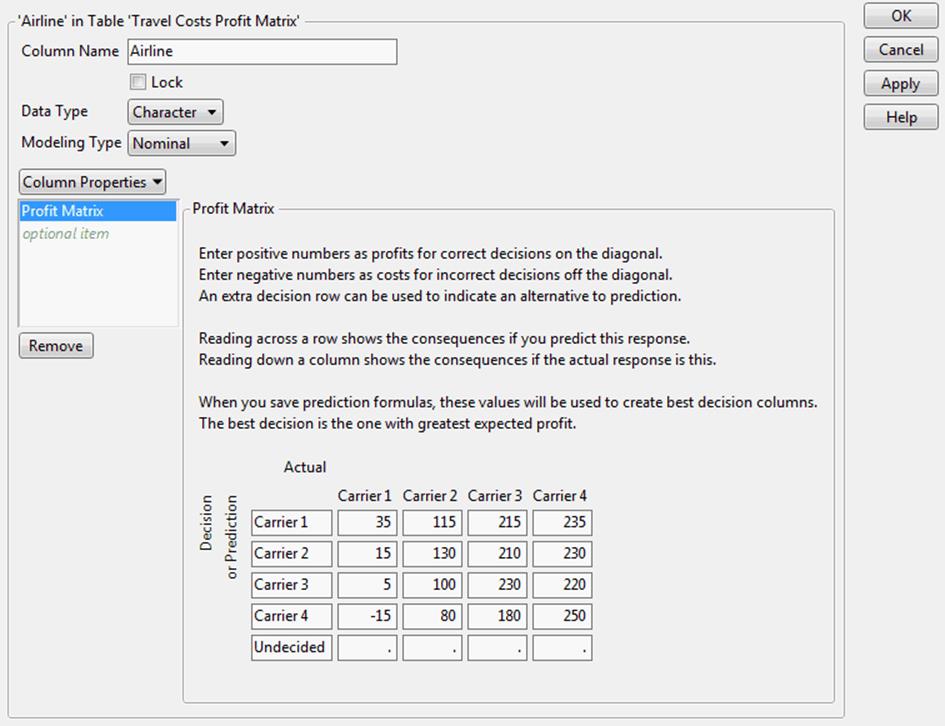
In a profit matrix, positive numbers represent projected profits from making sound and timely decisions. Negative numbers represent projected losses or costs resulting from making unprofitable or untimely decisions.

In a sample scenario, a travel agency uses four airlines to service its customers. The airlines range from Carrier 1, a low budget airline, up to Carrier 4, a luxury airline. The agency earns money by selling airline tickets to its customers. Depending on the carrier selected by the customer, the agency expects a certain amount of profit for each ticket sold. When the agency recommends a carrier, they reserve a ticket for a small fee (this is the prediction). If the customer decides to take the recommended carrier the agency profits by a certain amount less the reservation fee. However, if the customer decides to take a different carrier, the agency loses the reservation fee already paid and must purchase the alternate ticket and pay another reservation fee. As a result, the agency’s profit margin is less than predicted.

For example, the reservation fees for Carrier 1 through Carrier 4 are $15, $20, $30, and $50 respectively. The gross profits for a ticket sale for Carrier 1 through Carrier 4 are $50, $150, $260, and $300 respectively.

If the agency recommends Carrier 1 to a customer, who then decides to purchase a ticket, the agency reserves a ticket for $15 and then receives $50 for a net profit of $35. If the agency predicts that a customer will choose Carrier 1 but they instead choose Carrier 2, the agency must pay $15 for the Carrier 1 reservation and $20 for the actual reservation on Carrier 2. This gives the agency a net profit of $115. Conversely, if the agency predicts Carrier 4 but the customer decides on Carrier 1, the agency has a loss of $15.

Informative Missing

The Informative Missing column property directs most fitting platforms to use a coding system for columns that contain missing values. For continuous columns, the coding system consists of two columns. The first column is a column of the original values with missing values replaced by the mean of the nonmissing values; the second column is an indicator column to denote which rows are missing. For categorical columns, missing values are treated as a distinct level of the column.

Additional Properties

There are two additional properties: Expression Role and Other.

Expression Role

The Expression Role column property applies to columns containing expressions. It specifies whether the expression in the column should be interpreted as a Picture, a Matrix, or an Expression. The default is set to Picture. If the Expression Role is set to Picture and the expression is a picture, then the expression evaluates to a picture and the picture appears in the data table. Otherwise, the expression shows as a JSL expression. Change this setting to alter how expressions are used.

Note: Expression columns that contain images greater than 32KB in size are truncated when saved to Microsoft Excel. Those expression columns are not restored when imported back into JMP.

Select from the following options:

Picture

If the expression contains picture data, the column evaluates and the picture is displayed.

Matrix

If the expression contains a matrix, the column evaluates and the matrix is displayed. Otherwise, the data is displayed as an expression.

Expression

If the expression is simply an expression, use this option to display it in the column.

Use Expression when you want to work with an expression that might contain picture data, but you want to prevent JMP from displaying the image.

To drag images into an expression column:

1.Create a new column in a data table.

2.Double-click the column heading. Change the data type from Numeric to Expression.

3.ClickApply > OK.

4.Using your web browser, navigate to the website that contains the image that you want in your data table.

5.Select the image, and drag it into an empty cell in the Expression column.

Resize the cell to make the image larger.

To add an expression column using Summary:

1.Select Help > Sample Data Library and open CrimeData.jmp.

2.SelectTables > Summary.

3.SelectState, and clickGroup.

4.SelectTotal Rate, and clickStatistics > Histogram.

5.ClickOK.

A new data table appears that contains a new expression column with images of histograms. Resize the row to make images larger.

For more details about Summary, see Discovering JMP.

6.Right-click theHistogram(Total Rate)column, and selectColumn Info.

Notice the column’s data type is set to Expression.

7.SelectExpression Rolefrom the Column Properties menu.

The Expression Role is automatically set to Picture. In the rare case that a picture needs to be displayed as an Expression, change the setting to Expression.

8.ClickOK.

Expression Role is assigned to the Expression column.

Other

Use the Other column property to create your own column property and assign it any name that you choose. This property is then available for JSL programming.

1.Right-click on the column and select Column Properties > Other.

2.Enter a name for the new property.

3.Enter a value for the property.

Properties Assigned and Controlled by JMP

To control how information flows between platforms, JMP assigns some properties that you cannot control. These properties do not appear on the Column Properties menu.

Response Probability

In Profiler reports, the Response Probability property makes all levels of the categorical response variable appear in a single row. JMP automatically assigns the Response Probability property when certain probability formulas are saved to the data table. For example, the property is saved when the following steps are performed:

1.Fit a logistic regression model using the Fit Model platform.

2.Select theSave Probability Formulaoption in the report window.

JMP automatically assigns the Response Probability property to the new probability columns.

3.Select Prediction Profiler from the report’s red triangle menu.

The levels of the categorical response appear on the vertical axis. Probabilities for each level are shown.

Note: For more details, see the Profilers book.

Predicting

JMP automatically assigns the Predicting column property when you fit a model to a continuous response. The Predicting column property identifies the platform used to create the prediction formula. That platform is listed as the Creator in the Model Comparison platform.

Informative Missing Terms

Missing levels of a categorical variable are treated as informative missing in certain JMP platforms, either by default or if you request an informative missing fit. In these cases, JMP automatically assigns the Informative Missing Terms column property to a prediction formula column that includes the categorical variable. This column property ensures that the missing value category is treated as a distinct level of the categorical variable in plots and analyses that involve the prediction formula. In particular, profiler plots show the missing values as a level.

Standardize Attributes and Properties across Columns

A column might contain attributes (data types, modeling types, numeric formats, and so on) or properties (formulas, notes, list and range checks, and so on) that you want other columns to have. You can use the existing column to standardize the attributes and properties across columns. This includes both adding and deleting attributes and properties.

To apply an existing column’s attributes and properties to multiple columns

1.Select the column or columns containing the desired attributes or properties.

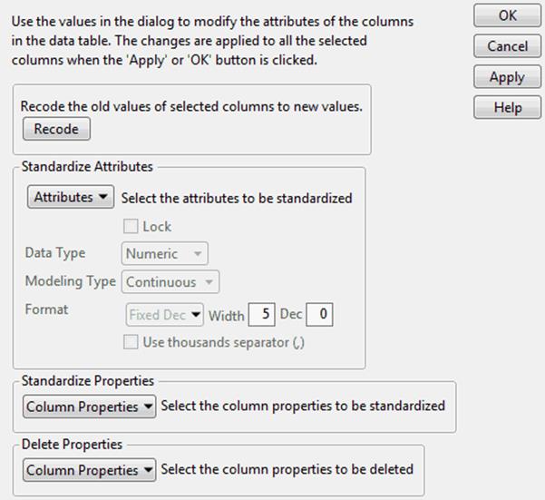
2.SelectCols > Standardize Attributes. The window inFigure 5.8appears.

Figure 5.8 Standardizing Attributes across Columns

Recode Values

Use the Recode option if you need to recode similar values within multiple columns in the same way. Once you click Recode, the values that appear are generated from the union of all of the selected columns. For example, suppose that you have two columns with user responses. One column contains the values Agree and Disagree. The other column contains the values Agree, Disagree, Unsure, and Strongly Disagree. You want to simplify all of the values in both columns to be A, D, U, and SD.

Note: If you want to recode values only in a single column, you can also use the Cols >Utilities > Recode option. See “View Patterns of Missing Data” in the “Enter and Edit Data” chapter.

Standardize Attributes

By default, the items within the Standardize Attributes panel are dimmed. To access an item, click the Attributes button and select the items to be duplicated across columns.

Note: The Input Format item is applicable only for the Date, Time, and Duration formats.

To change the values of any of the attributes, use the menus in the Standardize Attributes panel.

Standardize Properties

To standardize properties across columns

1.Select the columns that you want to standardize. One of those columns must contain the property that you want to add to the other columns.

2.SelectCols > Standardize Attributes.

3.SelectColumn Propertiesin the Standardize Properties area.

4.Select the property that you want to standardize. Modify the property settings if necessary.

5.ClickApplyto standardize the property across selected columns. Changes are shown in the data table, open reports, and open graphs.

Or click OK to standardize the property across selected columns and close the column properties window.

Delete Properties

To delete the same properties across multiple columns

1.Select the column containing the attributes or properties that you want to delete.

2.SelectCols > Standardize Attributes.

3.ClickColumn Propertiesin the Delete Properties area and select the properties that you want to delete.

4.ClickOK.

Example of Standardizing a Formula

If you have applied a formula to a column, and you want to apply that same formula to additional columns in the data table, use the Substitute Column Reference option.

Note: This option is dependent upon the location of the column that is referenced in the original formula. For example, if your original formula is based on the previous column, then any other formulas applied to additional columns are based on their previous columns.

For example, the Blood Pressure.jmp sample data table contains blood pressure measurements taken on five subjects three times each day, over a period of three days. You want to find the log of each blood pressure (BP) column.

1.Open the Blood Pressure.jmp sample data table.

Create nine new columns, one for each existing BP column.

2.SelectCols > Add Multiple Columns.

3.Add nine columns.

4.ClickOK.

Apply your original formula as follows:

5.Right-clickColumn 1and selectFormula.

6.SelectBP 8M.

7.SelectTranscendental > Log.

8.ClickOK.

Column 1 now contains the log of the BP 8M column. You want the rest of the empty columns to contain the log of the remainder of the BP columns.

9.In the data table, select all of the new columns that you created, including the one with the original formula (columns 1-9).

10.SelectCols > Standardize Attributes.

11.In the Standardize Properties panel, clickColumn Propertiesand selectFormula.

12.Select the check box next toSubstitute Column Reference.

13.ClickOK.

Now all of the new columns are populated with the log of the BP columns, in the order in which they appear. Column 1 contains the log for BP 8M, Column 2 contains the log for BP 12M, and so on.

Assign a Preselected Analysis Role

You can assign an analysis role, such as x, y, weight, or frequency, to a selected column and save the role with the data table. When you do this and then run an analysis, JMP uses the preselected role to automatically fill in the role boxes in windows. Then you do not have to specify these roles each time you run an analysis. For example, you might want a column named height to take the x role in every analysis of that data table. To enforce the x role, you assign the preselected role of x to the column.

When you select Freq, the values in that column are what JMP uses as the frequency of the observation. If n is the value of the Freq variable for a given row, then that row is used in computations n times. If it is less than 1 or is missing, then JMP does not use it to calculate any analyses.

When you select Weight, the values in that column provide weights for each observation in the data table. The variable does not have to be an integer, but it is included only in analyses when its value is greater than zero.

To assign a preselected role to a column

1.Highlight the column.

2.SelectCols > Preselect Role.

3.Select a role:No Role,X,Y,Weight, orFreq.

After you select the appropriate roles, icons in the Columns panel signify what roles have been assigned. Click the icon to access a list of roles and select a different one. See “Icons Representing Column Characteristics and Properties” in the “Get Started” chapter.