Large Scale Machine Learning with Python (2016)

Chapter 3. Fast SVM Implementations

Having experimented with online-style learning in the previous chapter, you may have been surprised by its simplicity yet effectiveness and scalability in comparison to batch learning. In spite of learning just one example at a time, SGD can approximate the results well as if all the data resides in the core memory and you were using a batch algorithm. All you need is that your stream be indeed stochastic (there are no trends in data) and that the learner is tuned well to the problem (the learning rate is often the key parameter to be fixed).

Anyway, examining such achievements closely, the results are still just comparable to batch linear models but not to learners that are more sophisticated and characterized by higher variance than bias, such as SVMs, neural networks, or bagging and boosting ensembles of decision trees.

For certain problems, such as tall and wide but sparse data, just linear combinations may be enough according to the observation that a simple algorithm with more data often wins over more complex ones trained on less data. Yet, even using linear models and by resorting to explicitly mapping existing features into higher-dimensionality ones (using different order of interactions, polynomial expansions, and kernel approximations), we can accelerate and improve the learning of complex nonlinear relationships between the response and features.

In this chapter, we will therefore first introduce linear SVMs as a machine learning algorithm alternative to linear models, powered by a different approach to the problem of learning from data. Then, we will demonstrate how we can create richer features from the existing ones in order to solve our machine learning tasks in a better way when facing large scale data, especially tall data (that is, datasets having many cases to learn from).

In summary, in this chapter, we will cover the following topics:

·        Introducing SVMs and providing you with the basic concepts and math formulas to figure out how they work

·        Proposing SGD with hinge loss as a viable solution for large scale tasks that uses the same optimization approach as the batch SVM

·        Suggesting nonlinear approximations to accompany SGD

·        Offering an overview of other large scale online solutions besides SGD algorithm made available by Scikit-learn

Datasets to experiment with on your own

As in the previous chapter, we will be using datasets from the UCI Machine Learning Repository, in particular the bike-sharing dataset (a regression problem) and Forest Covertype Data (a multiclass classification problem).

If you have not done so before or if you need to download both the datasets again, you will need a couple of functions defined in the Datasets to try the real thing yourself section of Chapter 2, Scalable Learning in Scikit-learn. The needed functions areunzip_from_UCI and gzip_from_UCI. Both have a Python connect to the UCI repository; download a compressed file and unzip it in the working Python directory. If you call the functions from an IPython cell, you will find the necessary new directories and files exactly where IPython will look for them.

In case the functions do not work for you, never mind; we will provide you with the link for a direct download. After that, all you will have to do is unpack the data in the current working Python directory, which you can discover by running the following command on your Python interface (IPython or any IDE):

In: import os

print "Current directory is: \"%s\"" % (os.getcwd())

Out: Current directory is: "C:\scisoft\WinPython-64bit-2.7.9.4\notebooks\Packt - Large Scale"

The bike-sharing dataset

The dataset comprises of two files in CSV format containing the hourly and daily count of bikes rented in the years between 2011 and 2012 within the Capital bike-share system in Washington D.C., USA. As a reminder, the data features the corresponding weather and seasonal information regarding the day of the rental.

The following code snippet will save the dataset on the local hard disk using the convenient unzip_from_UCI wrapper function:

In: UCI_url = 'https://archive.ics.uci.edu/ml/machine-learning-databases/00275/Bike-Sharing-Dataset.zip'

unzip_from_UCI(UCI_url, dest='bikesharing')

Out: Extracting in C:\scisoft\WinPython-64bit-2.7.9.4\notebooks\bikesharing

    unzipping day.csv

    unzipping hour.csv

If run successfully, the code will indicate in what directory the CSV files have been saved and print the names of both the unzipped files. If unsuccessful, just download the file from https://archive.ics.uci.edu/ml/machine-learning-databases/00275/Bike-Sharing-Dataset.zip and unzip the two files, day.csv and hour.csv, in a directory named bikesharing that you previously created in your Python working directory.

The covertype dataset

Donated by Jock A. Blackard, Dr. Denis J. Dean, Dr. Charles W. Anderson, and the Colorado State University, the covertype dataset contains 581,012 examples and a series of 54 cartographic variables, ranging from elevation to soil type, expected to be able to predict the forest cover type, which comprises seven kinds (so this is a multiclass problem). In order to assure comparability with academic studies on the same data, instructions recommend using the first 11,340 records for the training, the next 3,780 records for validation, and finally the remaining 565,892 records as test examples:

In: UCI_url = 'https://archive.ics.uci.edu/ml/machine-learning-databases/covtype/covtype.data.gz'

gzip_from_UCI(UCI_url)

In case of problems in running the code or if you prefer to prepare the file by yourself, just go to the UCI website, download the dataset from https://archive.ics.uci.edu/ml/machine-learning-databases/covtype/covtype.data.gz, and unpack it into the directory that Python is currently working on.

Support Vector Machines

Support Vector Machines (SVMs) are a set of supervised learning techniques for classification and regression (and also for outlier detection), which is quite versatile as it can fit both linear and nonlinear models thanks to the availability of special functions—kernel functions. The specialty of such kernel functions is to be able to map the input features into a new, more complex feature vector using a limited amount of computations. Kernel functions nonlinearly recombine the original features, making possible the mapping of the response by very complex functions. In such a sense, SVMs are comparable to neural networks as universal approximators, and thus can boast a similar predictive power in many problems.

Contrary to the linear models seen in the previous chapter, SVMs started as a method to solve classification problems, not regression ones.

SVMs were invented at the AT&T laboratories in the '90s by the mathematician, Vladimir Vapnik, and computer scientist, Corinna Cortes (but there are also many other contributors that worked with Vapnik on the algorithm). In essence, an SVM strives to solve a classification problem by finding a particular hyperplane separating the classes in the feature space. Such a particular hyperplane has to be characterized as being the one with the largest separating margin between the boundaries of the classes (the margin is to be intended as the gap, the space between the classes themselves, empty of any example).

Such intuition implies two consequences:

·        Empirically, SVMs try to minimize the test error by finding a solution in the training set that is exactly in the middle of the observed classes, thus the solution is clearly computational (it is an optimization based on quadratic programming—https://en.wikipedia.org/wiki/Quadratic_programming).

·        As the solution is based on just the boundaries of the classes as set by the adjoining examples (called the support vectors), the other examples can be ignored, making the technique insensible to outliers and less memory-intensive than methods based on matrix inversion such as linear models.

Given such a general overview on the algorithm, we will be spending a few pages pointing out the key formulations that characterize SVMs. Although a complete and detailed explanation of the method is beyond the scope of this book, sketching how it works can indeed help figure out what is happening under the hood of the technique and provide the foundation to understand how it can be made scalable to big data.

Historically, SVMs were thought as hard-margin classifiers, just like the perceptron. In fact, SVMs were initially set trying to find two hyperplanes separating the classes whose reciprocal distance was the maximum possible. Such an approach worked perfectly with linearly-separable synthetic data. Anyway, in the hard-margin version, when an SVM faced nonlinearly separable data, it could only succeed using nonlinear transformations of the features. However, they were always deemed to fail when misclassification errors were due to noise in data instead of non-linearity.

For such a reason, softmargins were introduced by means of a cost function that took into account how serious the error was (as hard margins kept track only if an error occurred), thus allowing a certain tolerance to misclassified cases whose error was not too big because they were placed next to the separating hyperplane.

Since the introduction of softmargins, SVMs also became able to withstand non-separability caused by noise. Softmargins were simply introduced by building the cost function around a slack variable that approximates the number of misclassified examples. Such a slack variable is also called the empirical risk (the risk of making a wrong classification as seen from the training data point of view).

In mathematical formulations, given a matrix dataset X of n examples and m features and a response vector expressing the belonging to a class in terms of +1 (belonging) and -1 (not belonging), a binary classification SVM strives to minimize the following cost function:

In the preceding function, w is the vector of coefficients that expresses the separating hyperplane together with the bias b, representing the offset from the origin. There is also lambda (λ>=0), which is the regularization parameter.

For a better understanding of how the cost function works, it is necessary to divide it into two parts. The first part is the regularization term:

The regularization term is contrasting the minimization process when the vector w assumes high values. The second term is called the loss term or slack variable, and actually is the core of the SVM minimization procedure:

The loss term outputs an approximate value of misclassification errors. In fact, the summation will tend to add a unit value for each classification error, whose total divided by n, the number of examples, will provide an approximate proportion of the classification error.

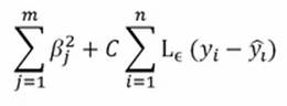
Often, as in the Scikit-learn implementation, the lambda is removed from the regularization term and replaced by a misclassification parameter C multiplying the loss term:

The relation between the previous parameter lambda and the new C is as follows:

It is just a matter of conventions, as the change from the parameter lambda to C on the optimization's formula doesn't imply different results.

The impact of the loss term is mediated by a hyperparameter C. High values of C impose a high penalization on errors, thus forcing the SVM to try to correctly classify all the training examples. Consequently, larger C values tend to force the margin to be tighter and take into consideration fewer support vectors. Such a reduction of the margin translates into an increased bias and reduced variance.

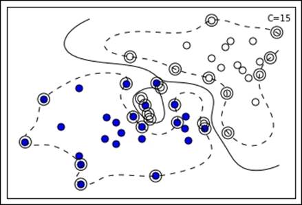
This leads us to specify the role of certain observations with respect to others; in fact, we define as support vectors those examples that are misclassified or not classified with confidence as they are inside the margin (noisy observations that make class separation impossible). Optimization is possible taking into account only such examples, making SVM a memory-efficient technique indeed:

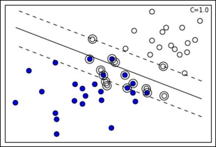
In the preceding visualization, you can notice the projection of two groups of points (blue and white) on two feature dimensions. An SVM solution with the C hyperparameter set to 1.0 can easily discover a separating line (in the plot represented as the continuous line), though there are some misclassified cases on both sides. In addition, the margin can be visualized (defined by the two dashed lines), being identifiable thanks to the support vectors of the respective class further from the separating line. In the chart, support vectors are marked by an external circle and you can actually notice that some support vectors are outside the margin; this is because they are misclassified cases and the SVM has to keep track of them for optimization purposes as their error is considered in the loss term:

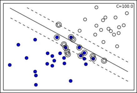
Increasing the C value, the margin tends to restrict as the SVM is taking into account fewer support vectors in the optimization process. Consequently, the slope of the separating line also changes.

On the contrary, smaller C values tend to relax the margin, thus increasing the variance. Extremely small C values can even lead the SVM to consider all the example points inside the margin. Smaller C values are ideal when there are many noisy examples. Such a setting forces the SVM to ignore many misclassified examples in the definition of the margin (Errors are weighted less, so they are tolerated more when searching for the maximum margin.):

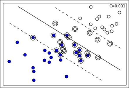
Continuing on the previous visual example, if we decrease the hyperparameter C, the margin actually expands because the number of the support vectors increases. Consequently, the margin being different, SVM resolves for a different separating line. There is no C value that can be deemed correct before being tested on data; the right value always has to be empirically found by cross-validation. By far, C is considered the most important hyperparameter in an SVM, to be set after deciding what kernel function to use.

Kernel functions instead map the original features into a higher-dimensional space by combining them in a nonlinear way. In such a way, apparently non-separable groups in the original feature space may turn separable in a higher-dimensional representation. Such a projection doesn't need too complex computations in spite of the fact that the process of explicitly transforming the original feature values into new ones can generate a potential explosion in the number of the features when projecting to high dimensionalities. Instead of doing such cumbersome computations, kernel functions can be simply plugged into the decision function, thus replacing the original dot product between the features and coefficient vector and obtaining the same optimization result as the explicit mapping would have had. (Such plugging is called the kernel trick because it is really a mathematical trick.)

Standard kernel functions are linear functions (implying no transformations), polynomial functions, radial basis functions (RBF), and sigmoid functions. To provide an idea, the RBF function can be expressed as follows:

Basically, RBF and the other kernels just plug themselves directly into a variant of the previously seen function to be minimized. The previously seen optimization function is called the primal formulation whereas the analogous re-expression is called the dual formulation:

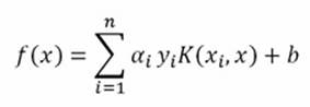
Though passing from the primal to the dual formulation is quite challenging without a mathematical demonstration, it is important to grasp that the kernel trick, given a kernel function that compares the examples by couples, is just a matter of a limited number of calculations with respect to the infinite dimensional feature space that it can unfold. Such a kernel trick renders the algorithm so particularly effective (comparable to neural networks) with respect to quite complex problems such as image recognition or textual classification:

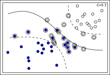
For instance, the preceding SVM solution is possible thanks to a sigmoid kernel, whereas the following one is due to an RBF one:

As visually noticeable, the RBF kernel allows quite complex definitions of the margin, even splitting it into multiple parts (and an enclave is noticeable in the preceding example).

The formulation of the RBF kernel is as follows:

Gamma is a hyperparameter for you to define a-priori. The kernel transformation creates some sort of classification bubbles around the support vectors, thus allowing the definition of very complex boundary shapes by merging the bubbles themselves.

The formulation of the sigmoid kernel is as follows:

Here, apart from gamma, r should be also chosen for the best result.

Clearly, solutions based on sigmoid, RBF, and polynomial, (Yes, it implicitly does the polynomial expansion that we will talk about in the following paragraphs.) kernels present more variance than the bias of the estimates, thus requiring a severe validation when deciding their adoption. Though an SVM is resistant to overfitting, it is not certainly immune to it.

Support vector regression is related to support vector classification. It varies just for the notation (more similar to a linear regression, using betas instead of a vector w of coefficients) and loss function:

Noticeably, the only significant difference is the loss function L-epsilon, which is insensitive to errors (thus not computing them) if examples are within a certain distance epsilon from the regression hyperplane. The minimization of such a cost function optimizes the result for a regression problem, outputting values and not classes.

Hinge loss and its variants

As concluding remarks about the inner nuts and bolts of an SVM, remember that the cost function at the core of the algorithm is the hinge loss:

As seen before, ŷ is expressed as the summation of the dot product of X and coefficient vector w with the bias b:

Reminiscent of the perceptron, such a loss function penalizes errors linearly, expressing an error when the example is classified on the wrong side of the margin, proportional to its distance from the margin itself. Though convex, having the disadvantage of not being differentiable everywhere, it is sometimes replaced by always differentiable variants such as the squared hinge loss (also called L2 loss whereas L1 loss is the hinge loss):

Another variant is the Huber loss, which is a quadratic function when the error is equal or below a certain threshold value h but a linear function otherwise. Such an approach mixes L1 and L2 variants of the hinge loss based on the error and it is an alternative quite resistant to outliers as larger error values are not squared, thus requiring fewer adjustments by the learning SVM. Huber loss is also an alternative to log loss (linear models) because it is faster to calculate and able to provide estimates of class probabilities (the hinge loss does not have such a capability).

From a practical point of view, there are no particular reports that Huber loss or L2 hinge loss can consistently perform better than hinge loss. In the end, the choice of a cost function just boils down to testing the available functions with respect to every different learning problem. (According to the principle of the no-free-lunch theorem, in machine learning, there are no solutions suitable for all the problems.)

Understanding the Scikit-learn SVM implementation

Scikit-learn offers an implementation of SVM using two C++ libraries (with a C API to interface with other languages) developed at the National Taiwan University, A Library for Support Vector Machines (LIBSVM) for SVM classification and regression (http://www.csie.ntu.edu.tw/~cjlin/libsvm/) and LIBLINEAR for classification problems using linear methods on large and sparse datasets (http://www.csie.ntu.edu.tw/~cjlin/liblinear/). Having both the libraries free to use, quite fast in computations, and already tested in quite a number of other solutions, all Scikit-learn implementations in the sklearn.svm module rely on one or the other, (The Perceptron and LogisticRegression classes also make use of them, by the way.) making Python just a convenient wrapper.

On the other hand, SGDClassifier and SGDRegressor use a different implementation as neither LIBSVM nor LIBLINEAR have an online implementation, both being batch learning tools. In fact, when operating, both LIBSVM and LIBLINEAR perform the best when allocated a suitable memory for kernel operations via the cache_size parameter.

The implementations for classification are as follows:

As for regression, the solutions are as follows:

As you can see, there are quite a few hyperparameters to be tuned for each version, making SVMs good learners when using default parameters and excellent ones when properly tuned by cross-validation, using GridSearchCV from the grid_search module in Scikit-learn.

As a golden rule, some parameters influence the result more and so should be fixed beforehand, others being dependent on their values. According to such an empirical rule, you have to correctly set the following parameters (ordered by rank of importance):

·        C: This is the penalty value that we discussed before. Decreasing it makes the margin larger, thus ignoring more noise but also making for more computations. A best value can be normally looked for in the np.logspace(-3, 3, 7) range.

·        kernel: This is the non-linearity workhorse because an SVM can be set to linear, poly, rbf, sigmoid, or a custom kernel (for experts!). The widely used one is certainly rbf.

·        degree: This works with kernel='poly', signaling the dimensionality of the polynomial expansion. It is ignored by other kernels. Usually, values from 2-5 work the best.

·        gamma: This is a coefficient for 'rbf', 'poly', and 'sigmoid'; high values tend to fit data in a better way. The suggested grid search range is np.logspace(-3, 3, 7).

·        nu: This is for regression and classification with nuSVR and nuSVC; this parameter approximates the training points that are not classified with confidence, misclassified points, and correct points inside or on the margin. It should be a number in the range [0,1] as it is a proportion relative to your training set. In the end, it acts as C with high proportions enlarging the margin.

·        epsilon: This parameter specifies how much error an SVR is going to accept by defining an epsilon large range where no penalty is associated with respect to the true value of the point. The suggested search range is np.insert(np.logspace(-4, 2, 7),0,[0]).

·        penalty, loss and dual: For LinearSVC, these parameters accept the ('l1','squared_hinge',False), ('l2','hinge',True), ('l2','squared_hinge',True), and ('l2','squared_hinge',False) combinations. The ('l2','hinge',True) combination is equivalent to theSVC(kernel='linear') learner.

As an example for basic classification and regression using SVC and SVR from Scikit-learn's sklearn.svm module, we will work with the Iris and Boston datasets, a couple of popular toy datasets (http://scikit-learn.org/stable/datasets/).

First, we will load the Iris dataset:

In: from sklearn import datasets

iris = datasets.load_iris()

X_i, y_i = iris.data, iris.target

Then, we will fit an SVC with an RBF kernel (C and gamma were chosen on the basis of other known examples in Scikit-learn) and test the results using the cross_val_score function:

from sklearn.svm import SVC

from sklearn.cross_validation import cross_val_score

import numpy as np

h_class = SVC(kernel='rbf', C=1.0, gamma=0.7, random_state=101)

scores = cross_val_score(h_class, X_i, y_i, cv=20, scoring='accuracy')

print 'Accuracy: %0.3f' % np.mean(scores)

Output: Accuracy: 0.969

The fitted model can provide you with an index pointing out what are the support vectors among your training examples:

In: h_class.fit(X_i,y_i)

print h_class.support_

Out: [ 13  14  15  22  24  41  44  50  52  56  60  62  63  66  68  70  72  76  77  83  84  85  98 100 106 110 114 117 118 119 121 123 126 127 129 131 133 134 138 141 146 149]

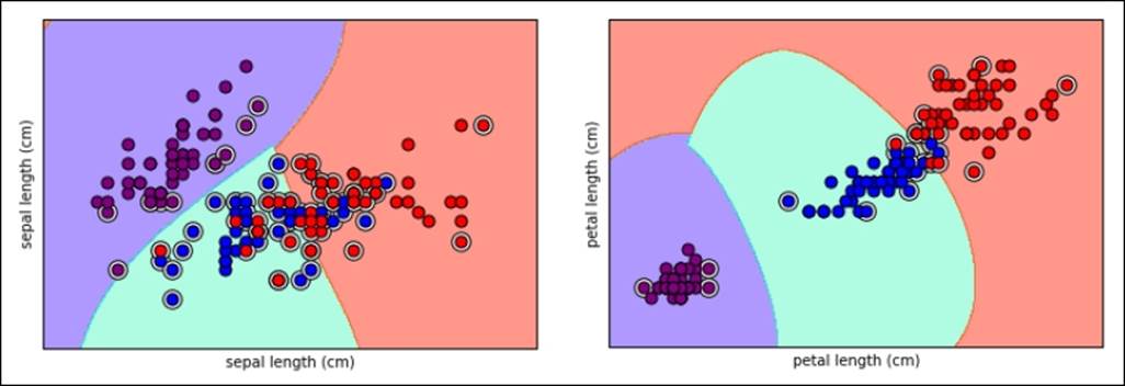
Here is a graphical representation of the support vectors selected by the SVC for the Iris dataset, represented with color decision boundaries (we tested a discrete grid of values in order to be able to project for each area of the chart what class the model will predict):

Tip

If you are interested in replicating the same charts, you can have a look and tweak this code snippet from http://scikit-learn.org/stable/auto_examples/svm/plot_iris.html.

To test an SVM regressor, we decided to try SVR with the Boston dataset. First, we upload the dataset in the core memory and then we randomize the ordering of examples as, noticeably, such a dataset is actually ordered in a subtle fashion, thus making results from not order-randomized cross-validation invalid:

In: import numpy as np

from sklearn.datasets import load_boston

from sklearn.preprocessing import StandardScaler

scaler = StandardScaler()

boston = load_boston()

shuffled = np.random.permutation(boston.target.size)

X_b = scaler.fit_transform(boston.data[shuffled,:])

y_b = boston.target[shuffled]

Tip

Due to the fact that we used the permutation function from the random module in the NumPy package, you may obtain a differently shuffled dataset and consequently a slightly different cross-validated score from the following test. Moreover, the features having different scales, it is a good practice to standardize the features so that they will have zero-centered mean and unit variance. Especially when using SVM with kernels, standardization is indeed crucial.

Finally, we can fit the SVR model (we decided on some C, gamma, and epsilon parameters that we know work fine) and, using cross-validation, we evaluate it by the root mean squared error:

In: from sklearn.svm import SVR

from sklearn.cross_validation import cross_val_score

h_regr = SVR(kernel='rbf', C=20.0, gamma=0.001, epsilon=1.0)

scores = cross_val_score(h_regr, X_b, y_b, cv=20, scoring='mean_squared_error')

print 'Mean Squared Error: %0.3f' % abs(np.mean(scores))

Out: Mean Squared Error: 28.087

Pursuing nonlinear SVMs by subsampling

SVMs have quite a few advantages over other machine learning algorithms:

·        They can handle majority of the supervised problems such as regression, classification, and anomaly detection, though they are actually best at binary classification.

·        They provide a good handling of noisy data and outliers and they tend to overfit less as they only work with support vectors.

·        They work fine with wide datasets (more features than examples); though, as with other machine learning algorithms, an SVM would gain both from dimensionality reduction and feature selection.

As drawbacks, we have to mention the following:

·        They provide just estimates, but no probabilities unless you run some time-consuming and computationally-intensive probability calibration by means of Platt scaling

·        They scale super-linearly with the number of examples

In particular, the last drawback puts a strong limitation on the usage of SVMs for large datasets. The optimization algorithm at the core of this learning technique—quadratic programming—scales in the Scikit-learn implementation between O(number of feature * number of samples^2) and O(number of feature * number of samples^3), a complexity that seriously limits the operability of the algorithm to datasets that are under 10^4 number of cases.

Again, as seen in the last chapter, there are just a few options when you give a batch algorithm and too much data: subsampling, parallelization, and out-of-core learning by streaming. Subsampling and parallelization are seldom quoted as the best solutions, streaming being the favored approach to implement SVMs with large-scale problems.

However, though less used, subsampling is quite easy to implement leveraging reservoir sampling, which can produce random samples rapidly from streams derived from datasets and infinite online streams. By subsampling, you can produce multiple SVM models, whose results can be averaged for better results. The predictions from multiple SVM models can even be stacked, thus creating a new dataset, and used to build a new model fusing the predictive capabilities of all, which will be described in Chapter 6, Classification and Regression Trees at Scale.

Reservoir sampling is an algorithm for randomly choosing a sample from a stream without having prior knowledge of how long the stream is. In fact, every observation in the stream has the same probability of being chosen. Initialized with a sample taken from the first observations in the stream, each element in the sample can be replaced at any moment by the example in the stream according to a probability proportional to the number of elements streamed up so far. So, for instance, when the i-th element of the stream arrives, it has a probability of being inserted in place of a random element in the sample. Such an insertion probability is equivalent to the sample dimension divided by i; therefore, it is progressively decreasing with respect to the stream length. If the stream is infinite, stopping at any time assures that the sample is representative of the elements seen so far.

In our example, we draw two random, mutually exclusive samples from the stream—one to train and one to test. We will extract such samples from the Covertype database, using the original ordered file. (As we will stream all the data before taking the sample, the random sampling won't be affected by the ordering.) We decided on a training sample of 5,000 examples, a number that should scale well on most desktop computers. As for the test set, we will be using 20,000 examples:

In: from random import seed, randint

SAMPLE_COUNT = 5000

TEST_COUNT   = 20000

seed(0) # allows repeatable results

sample = list()

test_sample = list()

for index, line in enumerate(open('covtype.data','rb')):

    if index < SAMPLE_COUNT:

        sample.append(line)

    else:

        r = randint(0, index)

        if r < SAMPLE_COUNT:

            sample[r] = line

        else:

            k = randint(0, index)

            if k < TEST_COUNT:

                if len(test_sample) < TEST_COUNT:

                    test_sample.append(line)

                else:

                    test_sample[k] = line

The algorithm should be streaming quite fast on the over 500,000 rows of the data matrix. In fact, we really did no preprocessing during the streaming in order to keep it the fastest possible. We consequently now need to transform the data into a NumPy array and standardize the features:

In: import numpy as np

from sklearn.preprocessing import StandardScaler

for n,line in enumerate(sample):

        sample[n] = map(float,line.strip().split(','))

y = np.array(sample)[:,-1]

scaling = StandardScaler()

X = scaling.fit_transform(np.array(sample)[:,:-1])

Once done with the training data X, y, we have to process the test data in the same way; particularly, we will have to standardize the features using standardization parameters (means and standard deviations) as in the training sample:

In: for n,line in enumerate(test_sample):

        test_sample[n] = map(float,line.strip().split(','))

yt = np.array(test_sample)[:,-1]

Xt = scaling.transform(np.array(test_sample)[:,:-1])

When both train and test sets are ready, we can fit the SVC model and predict the results:

In: from sklearn.svm import SVC

h = SVC(kernel='rbf', C=250.0, gamma=0.0025, random_state=101)

h.fit(X,y)

prediction = h.predict(Xt)

from sklearn.metrics import accuracy_score

print accuracy_score(yt, prediction)

Out: 0.75205

Achieving SVM at scale with SGD

Given the limitations of subsampling (first of all, the underfitting with respect to models trained on larger datasets), the only available option when using Scikit-learn for linear SVMs applied to large-scale streams remains the SGDClassifier and SGDRegressor methods, both available in the linear_model module. Let's see how to use them at their best and improve our results on the example datasets.

We are going to leverage the previous examples seen in the chapter for linear and logistic regression and transform them into an efficient SVM. As for classification, it is required that you set the loss type using the loss hyperparameter. The possible values for the parameter are 'hinge', 'squared_hinge', and 'modified_huber'. All such loss functions were previously introduced and discussed in this same chapter when dealing with the SVM formulation.

All of them imply applying a soft-margin linear SVM (no kernels), thus resulting in an SVM resistant to misclassifications and noisy data. However, you may also try to use the loss 'perceptron', a type of loss that results in a hinge loss without margin, a solution suitable when it is necessary to resort to a model with more bias than the other possible loss choices.

Two aspects have to be taken into account to gain the best results when using such a range of hinge loss functions:

·        When using any loss function, the stochastic gradient descent turns lazy, updating the vector of coefficients only when an example violates the previously defined margins. This is quite contrary to the loss function in the log or squared error, when actually every example is considered for the update of the coefficients' vector. In case there are many features involved in the learning, such a lazy approach leads to a resulting sparser vector of coefficients, thus reducing the overfitting. (A denser vector implies more overfitting because some coefficients are likely to catch more noise than signals from the data.)

·        Only the 'modified_huber' loss allows probability estimation, making it a viable alternative to the log loss (as found in the stochastic logistic regression). A modified Huber is also a better performer when dealing with multiclass one-vs-all (OVA) predictions as the probability outputs of the multiple models are better than the standard decision functions characteristic of hinge loss (probabilities work better than the raw output of the decision functions as they are on the same scale, bounded from 0 to 1). This loss function works by deriving a probability estimate directly from the decision function: (clip(decision_function(X), -1, 1) + 1) / 2.

As for regression problems, SGDRegressor offers two SVM loss options:

'epsilon_insensitive'

'squared_epsilon_insensitive'

Both activate a linear support vector regression, where errors (residual from the prediction) within the epsilon value are ignored. Past the epsilon value, the epsilon_insensitive loss considers the error as it is. The squared_epsilon_insensitive loss operates in a similar way though the error here is more penalizing as it is squared, with larger errors influencing the model building more.

In both cases, setting the correct epsilon hyperparameter is critical. As a default value, Scikit-learn suggests epsilon=0.1, but the best value for your problem has to be found by means of grid-search supported by cross-validation, as we will see in the next paragraphs.

Note that among regression losses, there is also a 'huber' loss available that does not activate an SVM kind of optimization but just modifies the usual 'squared_loss' to be insensible to outliers by switching from squared to linear loss past a distance of the value of the epsilon parameter.

As for our examples, we will be repeating the streaming process a certain number of times in order to demonstrate how to set different hyperparameters and transform features; we will use some convenient functions in order to reduce the number of repeated lines of code. Moreover, in order to speed up the execution of the examples, we will put a limit to the number of cases or tolerance values that the algorithm refers to. In such a way, both the training and validation times are kept at a minimum and no example will require you to wait more minutes than the time for a cup of tea or coffee.

As for the convenient wrapper functions, the first one will have the purpose to initially stream part or all the data once (we set a limit using the max_rows parameter). After completing the streaming, the function will be able to figure out all the categorical features' levels and record the different ranges of the numeric features. As a reminder, recording ranges is an important aspect to take care of. Both SGD and SVM are algorithms sensible to different range scales and they perform worse when working with a number outside the [-1,1] range.

As an output, our function will return two trained Scikit-learn objects: DictVectorizer (able to transform feature ranges present in a dictionary into a feature vector) and MinMaxScaler to rescale numeric variables in the [0,1] range (useful to keep values sparse in the dataset, thus keeping memory usage low and achieving fast computations when most values are zero). As a unique constraint, it is necessary for you to know the feature names of the numeric and categorical variables that you want to use for your predictive model. Features not enclosed in the lists' feed to the binary_features or numeric_features parameters actually will be ignored. When the stream has no features' names, it is necessary for you to name them using the fieldnames parameter:

In: import csv, time, os

import numpy as np

from sklearn.linear_model import SGDRegressor

from sklearn.feature_extraction import DictVectorizer

from sklearn.preprocessing import MinMaxScaler

from scipy.sparse import csr_matrix

def explore(target_file, separator=',', fieldnames= None, binary_features=list(), numeric_features=list(), max_rows=20000):

    """

    Generate from an online style stream a DictVectorizer and a MinMaxScaler.

    Parameters

----------

    target file = the file to stream from

    separator = the field separator character

    fieldnames = the fields' labels (can be omitted and read from file)

    binary_features = the list of qualitative features to consider

    numeric_features = the list of numeric futures to consider

    max_rows = the number of rows to be read from the stream (can be None)

    """

    features = dict()

    min_max  = dict()

    vectorizer = DictVectorizer(sparse=False)

    scaler = MinMaxScaler()

    with open(target_file, 'rb') as R:

        iterator = csv.DictReader(R, fieldnames, delimiter=separator)

        for n, row in enumerate(iterator):

            # DATA EXPLORATION

            for k,v in row.iteritems():

                if k in binary_features:

                    if k+'_'+v not in features:

                        features[k+'_'+v]=0

                elif k in numeric_features:

                    v = float(v)

                    if k not in features:

                        features[k]=0

                        min_max[k] = [v,v]

                    else:

                        if v < min_max[k][0]:

                            min_max[k][0]= v

                        elif v > min_max[k][1]:

                            min_max[k][1]= v

                else:

                    pass # ignore the feature

            if max_rows and n > max_rows:

                break

    vectorizer.fit([features])

    A = vectorizer.transform([{f:0 if f not in min_max else min_max[f][0] for f in vectorizer.feature_names_},

{f:1 if f not in min_max else min_max[f][1] for f in vectorizer.feature_names_}])

    scaler.fit(A)

    return vectorizer, scaler

Tip

This code snippet can be reused easily for your own machine learning applications for large-scale data. In case your stream is an online one (a continuous streaming) or a too long one, you can apply a different limit on the number of observed examples by setting the max_rows parameter.

The second function will instead just pull out the data from the stream and transform it into a feature vector, normalizing the numeric features if a suitable MinMaxScaler object is provided instead of a None setting:

In: def pull_examples(target_file, vectorizer, binary_features, numeric_features, target, min_max=None, separator=',',

fieldnames=None, sparse=True):

    """

    Reads a online style stream and returns a generator of normalized feature vectors

    Parameters

----------

    target file = the file to stream from

    vectorizer = a DictVectorizer object

    binary_features = the list of qualitative features to consider

    numeric_features = the list of numeric features to consider

    target = the label of the response variable

    min_max = a MinMaxScaler object, can be omitted leaving None

    separator = the field separator character

    fieldnames = the fields' labels (can be omitted and read from file)

    sparse = if a sparse vector is to be returned from the generator

    """

    with open(target_file, 'rb') as R:

        iterator = csv.DictReader(R, fieldnames, delimiter=separator)

        for n, row in enumerate(iterator):

            # DATA PROCESSING

            stream_row = {}

            response = np.array([float(row[target])])

            for k,v in row.iteritems():

                if k in binary_features:

                    stream_row[k+'_'+v]=1.0

                else:

                    if k in numeric_features:

                        stream_row[k]=float(v)

            if min_max:

                features = min_max.transform(vectorizer.transform([stream_row]))

            else:

                features = vectorizer.transform([stream_row])

            if sparse:

                yield(csr_matrix(features), response, n)

            else:

                yield(features, response, n)

Given these two functions, now let's try again to model the first regression problem seen in the previous chapter, the bike-sharing dataset, but using a hinge loss this time instead of the mean squared errors that we used before.

As the first step, we provide the name of the file to stream and a list of qualitative and numeric variables (as derived from the header of the file and initial exploration of the file). The code of our wrapper function will return some information on the hot-coded variables and value ranges. In this case, most of the variables will be binary ones, a perfect situation for a sparse representation, as most values in our dataset are plain zero:

In: source = '\\bikesharing\\hour.csv'

local_path = os.getcwd()

b_vars = ['holiday','hr','mnth', 'season','weathersit','weekday','workingday','yr']

n_vars = ['hum', 'temp', 'atemp', 'windspeed']

std_row, min_max = explore(target_file=local_path+'\\'+source, binary_features=b_vars, numeric_features=n_vars)

print 'Features: '

for f,mv,mx in zip(std_row.feature_names_, min_max.data_min_, min_max.data_max_):

    print '%s:[%0.2f,%0.2f] ' % (f,mv,mx)

Out:

Features:

atemp:[0.00,1.00]

holiday_0:[0.00,1.00]

holiday_1:[0.00,1.00]

...

workingday_1:[0.00,1.00]

yr_0:[0.00,1.00]

yr_1:[0.00,1.00]

As you can notice from the output, qualitative variables have been encoded using their variable name and adding, after an underscore character, their value and transformed into binary features (which has the value of one when the feature is present, otherwise it is set to zero). Note that we are always using our SGD models with the average=True parameter in order to assure a faster convergence (this corresponds to using the Averaged Stochastic Gradient Descent (ASGD) model as discussed in the previous chapter.):

In:from sklearn.linear_model import SGDRegressor

SGD = SGDRegressor(loss='epsilon_insensitive', epsilon=0.001, penalty=None, random_state=1, average=True)

val_rmse = 0

val_rmsle = 0

predictions_start = 16000

def apply_log(x): return np.log(x + 1.0)

def apply_exp(x): return np.exp(x) - 1.0

for x,y,n in pull_examples(target_file=local_path+'\\'+source,

                           vectorizer=std_row, min_max=min_max,

                           binary_features=b_vars, numeric_features=n_vars, target='cnt'):

    y_log = apply_log(y)

# MACHINE LEARNING

    if (n+1) >= predictions_start:

        # HOLDOUT AFTER N PHASE

        predicted = SGD.predict(x)

        val_rmse += (apply_exp(predicted) - y)**2

        val_rmsle += (predicted - y_log)**2

        if (n-predictions_start+1) % 250 == 0 and (n+1) > predictions_start:

            print n,

            print '%s holdout RMSE: %0.3f' % (time.strftime('%X'), (val_rmse / float(n-predictions_start+1))**0.5),

            print 'holdout RMSLE: %0.3f' % ((val_rmsle / float(n-predictions_start+1))**0.5)

    else:

        # LEARNING PHASE

        SGD.partial_fit(x, y_log)

print '%s FINAL holdout RMSE: %0.3f' % (time.strftime('%X'), (val_rmse / float(n-predictions_start+1))**0.5)

print '%s FINAL holdout RMSLE: %0.3f' % (time.strftime('%X'), (val_rmsle / float(n-predictions_start+1))**0.5)

Out:

16249 07:49:09 holdout RMSE: 276.768 holdout RMSLE: 1.801

16499 07:49:09 holdout RMSE: 250.549 holdout RMSLE: 1.709

16749 07:49:09 holdout RMSE: 250.720 holdout RMSLE: 1.696

16999 07:49:09 holdout RMSE: 249.661 holdout RMSLE: 1.705

17249 07:49:09 holdout RMSE: 234.958 holdout RMSLE: 1.642

07:49:09 FINAL holdout RMSE: 224.513

07:49:09 FINAL holdout RMSLE: 1.596

We are now going to try the classification problem of forest covertype:

In: source = 'shuffled_covtype.data'

local_path = os.getcwd()

n_vars = ['var_'+'0'*int(j<10)+str(j) for j in range(54)]

std_row, min_max = explore(target_file=local_path+'\\'+source, binary_features=list(),

                  fieldnames= n_vars+['covertype'], numeric_features=n_vars, max_rows=50000)

print 'Features: '

for f,mv,mx in zip(std_row.feature_names_, min_max.data_min_, min_max.data_max_):

    print '%s:[%0.2f,%0.2f] ' % (f,mv,mx)

Out:

Features:

var_00:[1871.00,3853.00]

var_01:[0.00,360.00]

var_02:[0.00,61.00]

var_03:[0.00,1397.00]

var_04:[-164.00,588.00]

var_05:[0.00,7116.00]

var_06:[58.00,254.00]

var_07:[0.00,254.00]

var_08:[0.00,254.00]

var_09:[0.00,7168.00]

...

After having sampled from the stream and fitted our DictVectorizer and MinMaxScaler objects, we can start our learning process using a progressive validation this time (the error measure is given by testing the model on the cases before they are used for the training), given the large number of examples available. Every certain number of examples as set by the sample variable in the code, the script reports the situation with average accuracy from the most recent examples:

In: from sklearn.linear_model import SGDClassifier

SGD = SGDClassifier(loss='hinge', penalty=None, random_state=1, average=True)

accuracy = 0

accuracy_record = list()

predictions_start = 50

sample = 5000

early_stop = 50000

for x,y,n in pull_examples(target_file=local_path+'\\'+source,

                           vectorizer=std_row,

                           min_max=min_max,

                           binary_features=list(), numeric_features=n_vars,

                           fieldnames= n_vars+['covertype'], target='covertype'):

    # LEARNING PHASE

    if n > predictions_start:

        accuracy += int(int(SGD.predict(x))==y[0])

        if n % sample == 0:

            accuracy_record.append(accuracy / float(sample))

            print '%s Progressive accuracy at example %i: %0.3f' % (time.strftime('%X'), n, np.mean(accuracy_record[-sample:]))

            accuracy = 0

    if early_stop and n >= early_stop:

            break

    SGD.partial_fit(x, y, classes=range(1,8))

Out: ...

19:23:49 Progressive accuracy at example 50000: 0.699

Tip

Having to process over 575,000 examples, we set an early stop to the learning process after 50,000. You are free to modify such parameters according to the power of your computer and time availability. Be warned that the code may take some time. We experienced about 30 minutes of computing on an Intel Core i3 processor clocking at 2.20 GHz.

Feature selection by regularization

In a batch context, it is common to operate feature selection by the following:

·        A preliminary filtering based on completeness (incidence of missing values), variance, and high multicollinearity between variables in order to have a cleaner dataset of relevant and operable features.

·        Another initial filtering based on the univariate association (chi-squared test, F-value, and simple linear regression) between the features and response variable in order to immediately remove the features that are of no use for the predictive task because they are little or not related to the response.

·        During modeling, a recursive approach inserting and/or excluding features on the basis of their capability to improve the predictive power of the algorithm, as tested on a holdout sample. Using a smaller subset of just relevant features allows the machine learning algorithm to be less affected by overfitting because of noisy variables and the parameters in excess due to the high dimensionality of the features.

Applying such approaches in an online setting is certainly still possible, but quite expensive in terms of the required time because of the quantity of data to stream to complete a single model. Recursive approaches based on a large number of iterations and tests require a nimble dataset that can fit in memory. As just previously quoted, in such a case, subsampling would be a good option in order to figure out features and models later to be applied to a larger scale.

Keeping on our out-of-core approach, regularization is the ideal solution as a way to select variables while streaming and filter out noisy or redundant features. Regularization works fine with online algorithms as it operates as the online machine learning algorithm is working and fitting its coefficients from the examples, without any need to run other streams for the purpose of selection. Regularization is, in fact, just a penalty value, which is added to the optimization of the learning process. It is dependent on the features' coefficient and a parameter named alpha setting the impact of regularization. The regularization balancing intervenes when coefficients' weights are updated by the model. At that time, regularization acts by reducing the resulting weights if the value of the update is not large enough. The trick of excluding or attenuating redundant variables is achieved because of the regularization alpha parameter, which has to be empirically set at the correct magnitude for the best result with respect to each specific data to be learned.

SGD implements the same regularization strategies to be found in batch algorithms:

·        L1 penalty pushing to zero redundant and not so important variables

·        L2 reducing the weight of less important features

·        Elastic Net mixing the effects of L1 and L2 regularization

L1 regularization is the perfect strategy when there are unusual and redundant variables as it will push the coefficients of such features to zero, making them irrelevant when calculating the prediction.

L2 is suitable when there are many correlations between the variables as its strategy is just to reduce the weights of the features whose variation is less important for the loss function minimization. With L2, all the variables keep on contributing to the prediction, though some less so.

Elastic Net mixes L1 and L2 using a weighted sum. This solution is interesting as sometimes L1 regularization is unstable when dealing with highly correlated variables, choosing one or the other with respect to the seen examples. Using ElasticNet, many unusual features will still be pushed to zero as in L1 regularization, but correlated ones will be attenuated as in L2.

Both SGDClassifier and SGDRegressor can implement L1, L2, and Elastic Net regularization using the penalty, alpha, and l1_ratio parameters.

Tip

The alpha parameter is the most critical parameter after deciding what kind of penalty or about the mix of the two. Ideally, you can test suitable values in the range from 0.1 to 10^-7, using the list of values produced by 10.0**-np.arange(1,7).

If penalty determinates what kind of regularization is chosen, alpha, as mentioned, will determinate its strength. As alpha is a constant that multiplies the penalization term; low alpha values will bring little influence on the final coefficient, whereas high values will significantly affect it. Finally, l1_ratio represents, when penalty='elasticnet', how much percentage is the L1 penalization with respect to L2.

Setting regularization with SGD is very easy. For instance, you may try changing the previous code example inserting a penalty L2 into SGDClassifier:

SGD = SGDClassifier(loss='hinge', penalty='l2', alpha= 0.0001, random_state=1, average=True)

If you prefer to test an Elastic-Net mixing the effects of the two regularization approaches, all you have to do is explicit the ratio between L1 and L2 by setting l1_ratio:

SGD = SGDClassifier(loss=''hinge'', penalty=''elasticnet'', \ alpha= 0.001, l1_ratio=0.5, random_state=1, average=True)

As the success of regularization depends on plugging the right kind of penalty and best alpha, regularization will be seen in action in our examples when dealing with the problem of hyperparameter optimization.

Including non-linearity in SGD

The fastest way to insert non-linearity into a linear SGD learner (and basically a no-brainer) is to transform the vector of the example received from the stream into a new vector including both power transformations and a combination of the features upto a certain degree.

Combinations can represent interactions between the features (explicating when two features concur to have a special impact on the response), thus helping the SVM linear model to include a certain amount of non-linearity. For instance, a two-way interaction is made by the multiplication of two features. A three-way is made by multiplying three features and so on, creating even more complex interactions for higher-degree expansions.

In Scikit-learn, the preprocessing module contains the PolynomialFeatures class, which can automatically transform the vector of features by polynomial expansion of the desired degree:

In: from sklearn.linear_model import SGDRegressor

from  sklearn.preprocessing import PolynomialFeatures

source = '\\bikesharing\\hour.csv'

local_path = os.getcwd()

b_vars = ['holiday','hr','mnth', 'season','weathersit','weekday','workingday','yr']

n_vars = ['hum', 'temp', 'atemp', 'windspeed']

std_row, min_max = explore(target_file=local_path+'\\'+source, binary_features=b_vars, numeric_features=n_vars)

poly = PolynomialFeatures(degree=2, interaction_only=False, include_bias=False)

SGD = SGDRegressor(loss='epsilon_insensitive', epsilon=0.001, penalty=None, random_state=1, average=True)

val_rmse = 0

val_rmsle = 0

predictions_start = 16000

def apply_log(x): return np.log(x + 1.0)

def apply_exp(x): return np.exp(x) - 1.0

for x,y,n in pull_examples(target_file=local_path+'\\'\

+source,vectorizer=std_row, min_max=min_max, \

sparse = False, binary_features=b_vars,\numeric_features=n_vars, target='cnt'):

    y_log = apply_log(y)

# Extract only quantitative features and expand them

    num_index = [j for j, i in enumerate(std_row.feature_names_) if i in n_vars]

    x_poly = poly.fit_transform(x[:,num_index])[:,len(num_index):]

    new_x = np.concatenate((x, x_poly), axis=1)

    # MACHINE LEARNING

    if (n+1) >= predictions_start:

        # HOLDOUT AFTER N PHASE

        predicted = SGD.predict(new_x)

        val_rmse += (apply_exp(predicted) - y)**2

        val_rmsle += (predicted - y_log)**2

        if (n-predictions_start+1) % 250 == 0 and (n+1) > predictions_start:

            print n,

            print '%s holdout RMSE: %0.3f' % (time.strftime('%X'), (val_rmse / float(n-predictions_start+1))**0.5),

            print 'holdout RMSLE: %0.3f' % ((val_rmsle / float(n-predictions_start+1))**0.5)

    else:

        # LEARNING PHASE

        SGD.partial_fit(new_x, y_log)

print '%s FINAL holdout RMSE: %0.3f' % (time.strftime('%X'), (val_rmse / float(n-predictions_start+1))**0.5)

print '%s FINAL holdout RMSLE: %0.3f' % (time.strftime('%X'), (val_rmsle / float(n-predictions_start+1))**0.5)

Out: ...

21:49:24 FINAL holdout RMSE: 219.191

21:49:24 FINAL holdout RMSLE: 1.480

Tip

PolynomialFeatures expects a dense matrix, not a sparse one as an input. Our pull_examples function allows the setting of a sparse parameter, which, normally set to True, can instead be set to False, thus returning a dense matrix as a result.

Trying explicit high-dimensional mappings

Though polynomial expansions are a quite powerful transformation, they can be computationally expensive when we are trying to expand to higher degrees and quickly contrast the positive effects of catching important non-linearity by overfitting caused by over-parameterization (when you have too many redundant and not useful features). As seen in SVC and SVR, kernel transformations can come to our aid. SVM kernel transformations, being implicit, require the data matrix in-memory in order to work. There is a class of transformations in Scikit-learn, based on random approximations, which, in the context of a linear model, can achieve very similar results as a kernel SVM.

The sklearn.kernel_approximation module contains a few such algorithms:

·        RBFSampler: This approximates a feature map of an RBF kernel

·        Nystroem: This approximates a kernel map using a subset of the training data

·        AdditiveChi2Sampler: This approximates feature mapping for an additive chi2 kernel, a kernel used in computer vision

·        SkewedChi2Sampler: This approximates feature mapping similar to the skewed chi-squared kernel also used in computer vision

Apart from the Nystroem method, none of the preceding classes require to learn from a sample of your data, making them perfect for online learning. They just need to know how an example vector is shaped (how many features there are) and then they will produce many random non-linearities that can, hopefully, fit well to your data problem.

There are no complex optimization algorithms to explain in these approximation algorithms; in fact, optimization itself is replaced by randomization and the results largely depend on the number of output features, pointed out by the n_components parameters. The more the output features, the higher the probability that by chance you'll get the right non-linearities working perfectly with your problem.

It is important to notice that, if chance has really such a great role in creating the right features to improve your predictions, then reproducibility of the results turns out to be essential and you should strive to obtain it or you won't be able to consistently retrain and tune your algorithm in the same way. Noticeably, each class is provided with a random_state parameter, thus allowing the controlling of random feature generation and being able to recreate it later on the same just as on different computers.

The theoretical fundamentals of such feature creation techniques are explained in the scientific articles, Random Features for Large-Scale Kernel Machines by A. Rahimi and Benjamin Recht (http://www.eecs.berkeley.edu/~brecht/papers/07.rah.rec.nips.pdf) andWeighted Sums of Random Kitchen Sinks: Replacing minimization with randomization in learning by A. Rahimi and Benjamin Recht (http://www.eecs.berkeley.edu/~brecht/papers/08.rah.rec.nips.pdf).

For our purposes, it will suffice to know how to implement the technique and have it contribute to improving our SGD models, both linear and SVM-based:

In: source = 'shuffled_covtype.data'

local_path = os.getcwd()

n_vars = ['var_'+str(j) for j in range(54)]

std_row, min_max = explore(target_file=local_path+'\\'+source, binary_features=list(),

                  fieldnames= n_vars+['covertype'], numeric_features=n_vars, max_rows=50000)

from sklearn.linear_model import SGDClassifier

from sklearn.kernel_approximation import RBFSampler

SGD = SGDClassifier(loss='hinge', penalty=None, random_state=1, average=True)

rbf_feature = RBFSampler(gamma=0.5, n_components=300, random_state=0)

accuracy = 0

accuracy_record = list()

predictions_start = 50

sample = 5000

early_stop = 50000

for x,y,n in pull_examples(target_file=local_path+'\\'+source,

                           vectorizer=std_row,

                           min_max=min_max,

                           binary_features=list(),

                           numeric_features=n_vars,

                           fieldnames= n_vars+['covertype'], target='covertype', sparse=False):

    rbf_x = rbf_feature.fit_transform(x)

    # LEARNING PHASE

    if n > predictions_start:

        accuracy += int(int(SGD.predict(rbf_x))==y[0])

        if n % sample == 0:

            accuracy_record.append(accuracy / float(sample))

            print '%s Progressive accuracy at example %i: %0.3f' % (time.strftime('%X'), n, np.mean(accuracy_record[-sample:]))

            accuracy = 0

    if early_stop and n >= early_stop:

            break

    SGD.partial_fit(rbf_x, y, classes=range(1,8))

Out: ...

07:57:45 Progressive accuracy at example 50000: 0.707

Hyperparameter tuning

As in batch learning, there are no shortcuts in out-of-core algorithms when testing the best combinations of hyperparameters; you need to try a certain number of combinations to figure out a possible optimal solution and use an out-of-sample error measurement to evaluate their performance.

As you actually do not know if your prediction problem has a simple smooth convex loss or a more complicated one and you do not know exactly how your hyperparameters interact with each other, it is very easy to get stuck into some sub-optimal local-minimum if not enough combinations are tried. Unfortunately, at the moment there are no specialized optimization procedures offered by Scikit-learn for out-of-core algorithms. Given the necessarily long time to train an SGD on a long stream, tuning the hyperparameters can really become a bottleneck when building a model on your data using such techniques.

Here, we present a few rules of thumb that can help you save time and efforts and achieve the best results.

First, you can tune your parameters on a window or a sample of your data that can fit in-memory. As we have seen with kernel SVMs, using a reservoir sample is quite fast even if your stream is huge. Then you can do your optimization in-memory and use the optimal parameters found on your stream.

As Léon Bottou from Microsoft Research has remarked in his technical paper, Stochastic Gradient Descent Tricks:

"The mathematics of stochastic gradient descent are amazingly independent of the training set size."

This is true for all the key parameters but especially for the learning rate; the learning rate that works better with a sample will work the best with the full data. In addition, the ideal number of passes over data can be mostly guessed by trying to converge on a small sampled dataset. As a rule of thumb, we report the indicative number of 10**6 examples examined by the algorithm—as pointed out by the Scikit-learn documentation—a number that we have often found accurate, though the ideal number of iterations may change depending on the regularization parameters.

Though most of the work can be done at a relatively small scale when using SGD, we have to define how to approach the problem of fixing multiple parameters. Traditionally, manual search and grid search have been the most used approaches, grid search solving the problem by systematically testing all the combinations of possible parameters at significant values (using, for instance, the log scale checking at the different power degree of 10 or of 2).

Recently, James Bergstra and Yoshua Bengio in their paper, Random Search for Hyper-Parameter Optimization, pointed out a different approach based on the random sampling of the values of the hyperparameters. Such an approach, though based on random choices, is often equivalent in results to grid search (but requiring fewer runs) when the number of hyperparameters is low and can exceed the performance of a systematic search when the parameters are many and not all of them are relevant for the algorithm performance.

We leave it to the reader to discover more reasons why this simple and appealing approach works so well in theory by referring to the previously mentioned paper by Bergstra and Bengio. In practice, having experienced its superiority with respect to other approaches, we propose an approach that works well for streams based on Scikit-learn's ParameterSampler function in the following example code snippet. ParameterSampler is able to randomly sample different sets of hyperparameters (both from distribution functions or lists of discrete values) to be applied to your learning SGD by means of the set_params method afterward:

In: from sklearn.linear_model import SGDRegressor

from sklearn.grid_search import ParameterSampler

source = '\\bikesharing\\hour.csv'

local_path = os.getcwd()

b_vars = ['holiday','hr','mnth', 'season','weathersit','weekday','workingday','yr']

n_vars = ['hum', 'temp', 'atemp', 'windspeed']

std_row, min_max = explore(target_file=local_path+'\\'+source, binary_features=b_vars, numeric_features=n_vars)

val_rmse = 0

val_rmsle = 0

predictions_start = 16000

tmp_rsmle = 10**6

def apply_log(x): return np.log(x + 1.0)

def apply_exp(x): return np.exp(x) - 1.0

param_grid = {'penalty':['l1', 'l2'], 'alpha': 10.0**-np.arange(2,5)}

random_tests = 3

search_schedule = list(ParameterSampler(param_grid, n_iter=random_tests, random_state=5))

results = dict()

for search in search_schedule:

    SGD = SGDRegressor(loss='epsilon_insensitive', epsilon=0.001, penalty=None, random_state=1, average=True)

    params =SGD.get_params()

    new_params = {p:params[p] if p not in search else search[p] for p in params}

    SGD.set_params(**new_params)

    print str(search)[1:-1]

    for iterations in range(200):

        for x,y,n in pull_examples(target_file=local_path+'\\'+source,

                                   vectorizer=std_row, min_max=min_max, sparse = False,

                                   binary_features=b_vars, numeric_features=n_vars, target='cnt'):

            y_log = apply_log(y)

# MACHINE LEARNING

            if (n+1) >= predictions_start:

                # HOLDOUT AFTER N PHASE

                predicted = SGD.predict(x)

                val_rmse += (apply_exp(predicted) - y)**2

                val_rmsle += (predicted - y_log)**2

            else:

                # LEARNING PHASE

                SGD.partial_fit(x, y_log)

        examples = float(n-predictions_start+1) * (iterations+1)

        print_rmse = (val_rmse / examples)**0.5

        print_rmsle = (val_rmsle / examples)**0.5

        if iterations == 0:

            print 'Iteration %i - RMSE: %0.3f - RMSE: %0.3f' % (iterations+1, print_rmse, print_rmsle)

        if iterations > 0:

            if tmp_rmsle / print_rmsle <= 1.01:

                print 'Iteration %i - RMSE: %0.3f - RMSE: %0.3f\n' % (iterations+1, print_rmse, print_rmsle)

                results[str(search)]= {'rmse':float(print_rmse), 'rmsle':float(print_rmsle)}

                break

        tmp_rmsle = print_rmsle

Out:

'penalty': 'l2', 'alpha': 0.001

Iteration 1 - RMSE: 216.170 - RMSE: 1.440

Iteration 20 - RMSE: 152.175 - RMSE: 0.857

'penalty': 'l2', 'alpha': 0.0001

Iteration 1 - RMSE: 714.071 - RMSE: 4.096

Iteration 31 - RMSE: 184.677 - RMSE: 1.053

'penalty': 'l1', 'alpha': 0.01

Iteration 1 - RMSE: 1050.809 - RMSE: 6.044

Iteration 36 - RMSE: 225.036 - RMSE: 1.298

The code leverages the fact that the bike-sharing dataset is quite small and doesn't require any sampling. In other contexts, it makes sense to limit the number of treated rows or create a smaller sample before by means of reservoir sampling or other sampling techniques for streams seen so far. If you would like to explore optimization in more depth, you can change the random_tests variable, fixing the number of sampled hyperparameters' combinations to be tested. Then, you modify the if tmp_rmsle / print_rmsle <= 1.01condition using a number nearer to 1.0—if not 1.0 itself—thus letting the algorithm fully converge until some possible gain in predictive power is feasible.

Tip

Though it is recommended to use distribution functions rather than picking from lists of values, you can still appropriately use the hyperparameters' ranges that we suggested before by simply enlarging the number of values to be possibly picked from the lists. For instance, for alpha in L1 and L2 regularization, you could use NumPy's function, arrange, with a small step such as 10.0**-np.arange(1, 7, step=0.1), or use NumPy logspace with a high number for the num parameter: 1.0/np.logspace(1,7,num=50).

Other alternatives for SVM fast learning

Though the Scikit-learn package provides enough tools and algorithms to learn out-of-core, there are other interesting alternatives among free software. Some are based on the same libraries that Scikit-learn itself uses, such as the Liblinear/SBM and others are completely new, such as sofia-ml, LASVM and Vowpal Wabbit. For instance, Liblinear/SBMis based on selective block minimization and implemented as a fork liblinear-cdblock of the original library (https://www.csie.ntu.edu.tw/~cjlin/libsvmtools/#large_linear_classification_when_data_cannot_fit_in_memory). Liblinear/SBM achieves to fit nonlinear SVMs on large amounts of data that cannot fit in-memory using the trick of training the learner using new samples of data and mixing it with previous samples already used for minimization (hence the blocked term in the name of the algorithm).

SofiaML (https://code.google.com/archive/p/sofia-ml/) is another alternative. SofiaML is based on an online SVM optimization algorithm called Pegasos SVM. This algorithm is an online SVM approximation, just as another software called LaSVM created by Leon Bottou (http://leon.bottou.org/projects/lasvm). All these solutions can work with sparse data, especially textual, and solve regression, classification, and ranking problems. To date, no alternative solution that we tested proved as fast and versatile as Vowpal Wabbit, the software that we are going to present in the next sections and use to demonstrate how to integrate external programs with Python.

Nonlinear and faster with Vowpal Wabbit

Vowpal Wabbit (VW) is an open source project for a fast online learner initially released in 2007 by John Langford, Lihong Li, and Alex Strehl from Yahoo! Research (http://hunch.net/?p=309) and then successively sponsored by Microsoft Research, as John Langford became the principal researcher at Microsoft. The project has developed over the years, arriving today at version 8.1.0 (at the time this chapter was written), with almost one hundred contributors working on it. (For a visualization of the development of the contributions over time, there is an interesting video using the software Gource at https://www.youtube.com/watch?v=-aXelGLMMgk.). To date, VW is still being constantly developed and keeps on increasing its learning capabilities at each development iteration.

The striking characteristic of VW is that it is very fast compared to other solutions available (LIBLINEAR, Sofia-ml, svmsgd, and Scikit-learn). Its secret is simple, yet extremely effective: it can load data and learn from it at the same time. An asynchronous thread does the parsing of the examples flowing in as a number of learning threads work on a disjoint set of features, thus assuring a high computational efficiency even when parsing involves high-dimensional feature creation (such as quadratic or cubic polynomial expansion). In most cases, the real bottleneck of the learning process is the transmission bandwidth of the disk or network transmitting the data to VW.

VW can work out classification (even multiclass and multilabel), regression (OLS and quantile), and active learning problems, offering a vast range of accompanying learning tools (called reductions) such as matrix factorization, Latent Dirichlet Allocation (LDA), neural networks, n-grams for language models, and bootstrapping.

Installing VW

VW can be retrieved from the online versioning repository GitHub (https://github.com/JohnLangford/vowpal_wabbit), where it can be Git-cloned or just downloaded in the form of a packed zip. Being developed on Linux systems, it is easily compiled on any POSIX environment by a simple sequence of make and make install commands. Detailed instructions for installation are available directly on its installation page and you can download Linux precompiled binaries directly from the author (https://github.com/JohnLangford/vowpal_wabbit/wiki/Download).

A VW version working on Windows operating systems, unfortunately, is a bit more difficult to obtain. In order to create one, the first reference is the documentation itself of VW where a compiling procedure is explained in detail (https://github.com/JohnLangford/vowpal_wabbit/blob/master/README.windows.txt).

Tip

On the accompanying website of the book, we will provide both 32-bit and 64-bit Windows binaries of the 8.1.0 version of VW that we have used for the book.

Understanding the VW data format

VW can work with a particular data format and is invoked from a shell. John Langford uses this sample dataset for his online tutorial (https://github.com/JohnLangford/vowpal_wabbit/wiki/Tutorial), representing three houses whose roofs could be replaced. We find it interesting proposing it to you and commenting on it together:

In:

with open('house_dataset','wb') as W:

    W.write("0 | price:.23 sqft:.25 age:.05 2006\n")

    W.write("1 2 'second_house | price:.18 sqft:.15 age:.35 1976\n")

    W.write("0 1 0.5 'third_house | price:.53 sqft:.32 age:.87 1924\n")

with open('house_dataset','rb') as R:

    for line in R:

        print line.strip()

Out:

0 | price:.23 sqft:.25 age:.05 2006

1 2 'second_house | price:.18 sqft:.15 age:.35 1976

0 1 0.5 'third_house | price:.53 sqft:.32 age:.87 1924

The first noticeable aspect of the file format is that it doesn't have a header. This is because VW uses the hashing trick to allocate the features into a sparse vector, therefore knowing in advance the features that are not necessary at all. Data blocks are divided by pipes (the character|) into namespaces, to be intended as different clusters of features, each one containing one or more features.

The first namespace is always the one containing the response variable. The response can be a real number (or an integer) pointing out a numeric value to be regressed, a binary class, or a class among multiple ones. The response is always the first number to be found on a line. A binary class can be encoded using 1 for positive and -1 for negative (using 0 as a response is allowed only for regression). Multiple classes should be numbered from 1 onward and having gap numbers is not advisable because VW asks for the last class and considers all the integers between 1 and the last one.

The number immediately after the response value is the weight (telling you if you have to consider an example as a multiple example or as a fraction of one), then the base, which plays the role of the initial prediction (a kind of bias). Finally, preceded by the apostrophe character ('), there is the label, which can be a number or text to be later found in the VW outputs (in a prediction, you have an identifier for every estimation). Weight, base, and labels are not compulsory: if omitted, weight will be imputed as 1 and base and label won't matter.

Following the first namespace, you can add as many namespaces as you want, labeling each one by a number or string. In order to be considered the label of the namespace, it should be stuck to the pipe, for instance, |label.

After the label of the namespace, you can add any feature by its name. The feature name can be anything, but should contain a pipe or colon. You can just put entire texts in the namespaces and every word will be treated as a feature. Every feature will be considered valued as 1. If you want to assign a different number, just stick a colon at the end of the feature name and put its value after it.

For instance, a valid row readable by Vowpal Wabbit is:

0 1 0.5 'third_house | price:.53 sqft:.32 age:.87 1924

In the first namespace, the response is 0, the example weights 1, the base is 0.5, and its label is third_house. The namespace is nameless and is constituted by four features such as price (value is .53), sqft (value is .32), age (value is .87), and 1924 (value is 1).

If you have a feature in an example but not in another one, the algorithm will pretend that the feature value is zero in the second example. Therefore, a feature such as 1924 in the preceding example can be intended as a binary variable as, when it is present, it is automatically valued 1, when missing 0. This also tells you how VW handles missing values—it automatically considers them as 0 values.

Tip

You can easily handle missing values by putting a new feature when a value is missing. If the feature is age, for instance, you can add a new feature, age_missing, which will be a binary variable having value as 1. When estimating the coefficients, this variable will act as a missing value estimator.

On the author's website, you can also find an input validator, verifying that your input is correct for VW and displaying how it is interpreted by the software:

http://hunch.net/~vw/validate.html

Python integration

There are a few packages integrating it with Python (vowpal_porpoise, Wabbit Wappa, or pyvw) and installing them is easy in Linux systems, but much harder on Windows. No matter whether you are working with Jupyter or IDE, the easiest way to use VW integrated with Python's scripts is to leverage the Popen function from the subprocess package. That makes VW run in parallel with Python. Python just waits for VW to complete its operation by capturing its output and printing it on the screen:

In: import subprocess

def execute_vw(parameters):

    execution = subprocess.Popen('vw '+parameters, \

                shell=True, stderr=subprocess.PIPE)

    line = ""

    history = ""

    while True:

        out = execution.stderr.read(1)

        history += out

        if out == '' and execution.poll() != None:

            print '------------ COMPLETED ------------\n'

            break

        if out != '':

            line += out

            if '\n' in line[-2:]:

                print line[:-2]

                line = ''

    return history.split('\r\n')

The functions return a list of the outputs of the learning process, making it easy to process it, extracting relevant reusable information (like the error measure). As a precondition for its correct functioning, place the VW executable (the vw.exe file) in the Python working directory or system path where it can be found.

By invoking the function on the previously recorded housing dataset, we can have a look at how it works and what outputs it produces:

In:

params = "house_dataset"

results = execute_vw(params)

Out:

Num weight bits = 18

learning rate = 0.5

initial_t = 0

power_t = 0.5

using no cache

Reading datafile = house_dataset

num sources = 1

average  since         example        example  current  current  current

loss     last          counter         weight    label  predict features

0.000000 0.000000            1            1.0   0.0000   0.0000        5

0.666667 1.000000            2            3.0   1.0000   0.0000        5

finished run

number of examples per pass = 3

passes used = 1

weighted example sum = 4.000000

weighted label sum = 2.000000

average loss = 0.750000

best constant = 0.500000

best constant's loss = 0.250000

total feature number = 15

------------ COMPLETED ------------

The initial rows of the output just recall the used parameters and provide confirmation of which data file is being used. Most interesting is the progressive reported by the number of streamed examples (reported by the power of 2, so example 1, 2, 4, 8, 16, and so on). With respect to the loss function, an average loss measure is reported, progressive for the first iteration, based on the hold-out set afterward, whose loss is signaled by postponing the letter h (if holding out is excluded, it is possible that just the in-sample measure is reported). On the example weight column, the weight of the example is reported and then the example is furthermore described as current label, current predict and displays the number of features found on that line (current features). All such information should help you keep an eye on the stream and learning process.

After the learning is completed, a few reporting measures are reported. The average loss is the most important, in particular when a hold-out is used. Using such loss is most useful for comparative reasons as it can be immediately compared with best constant's loss (the baseline predictive power of a simple constant) and with different runs using different parameter configurations.

Another very useful function to integrate VW and Python is a function that we prepared automatically converting CSV files to VW data files. You can find it in the following code snippet. It will help us replicate the previous bike-sharing and covertype problems using VW this time, but it can be easily reused for your own projects:

In: import csv

def vw_convert(origin_file, target_file, binary_features, numeric_features, target, transform_target=lambda(x):x,

               separator=',', classification=True, multiclass=False, fieldnames= None, header=True, sparse=True):

    """

    Reads a online style stream and returns a generator of normalized feature vectors

    Parameters

----------

    original_file = the CSV file you are taken the data from

    target file = the file to stream from

    binary_features = the list of qualitative features to consider

    numeric_features = the list of numeric features to consider

    target = the label of the response variable

    transform_target = a function transforming the response

    separator = the field separator character

    classification = a Boolean indicating if it is classification

    multiclass =  a Boolean for multiclass classification

    fieldnames = the fields' labels (can be omitted and read from file)

    header = a boolean indicating if the original file has an header

    sparse = if a sparse vector is to be returned from the generator

    """

    with open(target_file, 'wb') as W:

        with open(origin_file, 'rb') as R:

iterator = csv.DictReader(R, fieldnames, delimiter=separator)

            for n, row in enumerate(iterator):

                if not header or n>0:

                # DATA PROCESSING

                    response = transform_target(float(row[target]))

                    if classification and not multiclass:

                            if response == 0:

                                stream_row = '-1 '

                            else:

                                stream_row = '1 '

                    else:

                        stream_row = str(response)+' '

                    quantitative = list()

                    qualitative  = list()

                    for k,v in row.iteritems():

                        if k in binary_features:

                            qualitative.append(str(k)+\

'_'+str(v)+':1')

                        else:

                            if k in numeric_features and (float(v)!=0 or not sparse):

                                quantitative.append(str(k)+':'+str(v))

if quantitative:

                        stream_row += '|n '+\

' '.join(quantitative)

                    if qualitative:

                        stream_row += '|q '+\

' '.join(qualitative)

W.write(stream_row+'\n')

A few examples using reductions for SVM and neural nets

VW works on minimizing a general cost function, which is as follows:

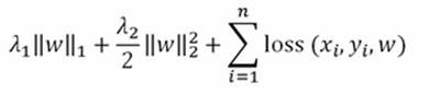
As in other formulations seen before, w is the coefficient vector and the optimization is obtained separately for each xi and yi according to the chosen loss function (OLS, logistic, or hinge). Lambda1 and lambda2 are the regularization parameters that, by default, are zero but can be set using the --l1 and --l2 options in the VW command line.

Given such a basic structure, VW has been made more complex and complete over time using the reduction paradigm. A reduction is just a way to reuse an existing algorithm in order to solve new problems without coding new solving algorithms from scratch. In other words, if you have a complex machine learning problem A, you just reduce it to B. Solving B hints at a solution of A. This is also justified by the growing interest in machine learning and the exploding number of problems that cannot be solved creating hosts of new algorithms. It is an interesting approach leveraging the existing possibilities offered by basic algorithms and the reason why VW has grown its applicability over time though the program has stayed quite compact. If you are interested in this approach, you can have a look at these two tutorials from John Langford: http://hunch.net/~reductions_tutorial/ and http://hunch.net/~jl/projects/reductions/reductions.html.

For other illustration purposes, we will briefly introduce you to a couple of reductions to implement an SVM with an RBFkernel and a shallow neural network using VW in a purely out-of-core way. We will be using some toy datasets for the purpose.

Here is the Iris dataset, changed to a binary classification problem to guess the Iris Versicolor from the Setosa and Virginica:

In: import numpy as np

from sklearn.datasets import load_iris, load_boston

from random import seed

iris = load_iris()

seed(2)

re_order = np.random.permutation(len(iris.target))

with open('iris_versicolor.vw','wb') as W1:

    for k in re_order:

        y = iris.target[k]

        X = iris.values()[1][k,:]

        features = ' |f '+' '.join([a+':'+str(b) for a,b in zip(map(lambda(a): a[:-5].replace(' ','_'), iris.feature_names),X)])

        target = '1' if y==1 else '-1'

        W1.write(target+features+'\n')

Then for a regression problem, we will be using the Boston house pricing dataset:

In: boston = load_boston()

seed(2)

re_order = np.random.permutation(len(boston.target))

with open('boston.vw','wb') as W1:

     for k in re_order:

        y = boston.target[k]

        X = boston.data[k,:]

        features = ' |f '+' '.join([a+':'+str(b) for a,b in zip(map(lambda(a): a[:-5].replace(' ','_'), iris.feature_names),X)])

        W1.write(str(y)+features+'\n')

First, we will be trying SVM. kvsm is a reduction based on the LaSVM algorithm (Fast Kernel Classifiers with Online and Active Learning—http://www.jmlr.org/papers/volume6/bordes05a/bordes05a.pdf) without a bias term. The VW version typically works in just one pass and with a 1-2 reprocessing of a randomly picked support vector (though some problems may need multiple passes and reprocessing). In our case, we are just using a single pass and a couple of reprocessings in order to fit an RBF kernel on our binary problem (KSVM works only for classification problems). Implemented kernels are linear, radial basis function, and polynomial. In order to have it work, use the --ksvm option, set a number for reprocessing (default is 1) by --reprocess, choose the kernel with --kernel(options are linear, poly, and rbf). Then, if the kernel is polynomial, set an integer number for --degree, or a float (default is 1.0) for --bandwidth if you are using RBF. You also have to compulsorily specify l2 regularization; otherwise, the reduction won't work properly. In our example, we make an RBFkernel with bandwidth 0.1:

In: params = '--ksvm --l2 0.000001 --reprocess 2 -b 18 --kernel rbf --bandwidth=0.1 -p iris_bin.test -d iris_versicolor.vw'

results = execute_vw(params)

accuracy = 0

with open('iris_bin.test', 'rb') as R:

    with open('iris_versicolor.vw', 'rb') as TRAIN:

        holdouts = 0.0

        for n,(line, example) in enumerate(zip(R,TRAIN)):

            if (n+1) % 10==0:

                predicted = float(line.strip())

                y = float(example.split('|')[0])

                accuracy += np.sign(predicted)==np.sign(y)

                holdouts += 1           

print 'holdout accuracy: %0.3f' % ((accuracy / holdouts)**0.5)

Out: holdout accuracy: 0.966

Neural networks are another cool addition to VW; thanks to the work of Paul Mineiro (http://www.machinedlearnings.com/2012/11/unpimp-your-sigmoid.html), VW can implement a single-layer neural network with hyperbolic tangent (tanh) activation and, optionally, dropout (using the --dropout option). Though it is only possible to decide the number of neurons, the neural reduction works fine with both regression and classification problems and can smoothly take on other transformations by VW as inputs (such as quadratic variables and n-grams), making it a very well-integrated, versatile (neural networks can solve quite a lot of problems), and fast solution. In our example, we apply it to the Boston dataset using five neurons and dropout:

In: params = 'boston.vw -f boston.model --loss_function squared -k --cache_file cache_train.vw --passes=20 --nn 5 --dropout'

results = execute_vw(params)

params = '-t boston.vw -i boston.model -k --cache_file cache_test.vw -p boston.test'

results = execute_vw(params)

val_rmse = 0

with open('boston.test', 'rb') as R:

    with open('boston.vw', 'rb') as TRAIN:

        holdouts = 0.0

        for n,(line, example) in enumerate(zip(R,TRAIN)):

            if (n+1) % 10==0:

                predicted = float(line.strip())

                y = float(example.split('|')[0])

                val_rmse += (predicted - y)**2

                holdouts += 1            

print 'holdout RMSE: %0.3f' % ((val_rmse / holdouts)**0.5)

Out: holdout RMSE: 7.010

Faster bike-sharing

Let's try VW on the previously created bike-sharing example file in order to explain the output components. As the first step, you have to transform the CSV file into a VW file and the previous vw_convert function will come in handy doing this. As before, we will apply a logarithmic transformation on the numeric response, using the apply_log function passed by the transform_target parameter of the vw_convert function:

In: import os

import numpy as np

def apply_log(x):

    return np.log(x + 1.0)

def apply_exp(x):

    return np.exp(x) - 1.0

local_path = os.getcwd()

b_vars = ['holiday','hr','mnth', 'season','weathersit','weekday','workingday','yr']

n_vars = ['hum', 'temp', 'atemp', 'windspeed']

source = '\\bikesharing\\hour.csv'

origin = target_file=local_path+'\\'+source

target = target_file=local_path+'\\'+'bike.vw'

vw_convert(origin, target, binary_features=b_vars, numeric_features=n_vars, target = 'cnt', transform_target=apply_log,

               separator=',', classification=False, multiclass=False, fieldnames= None, header=True)

After a few seconds, the new file should be ready. We can immediately run our solution, which is a simple linear regression (the default option in VW). The learning is expected to run for 100 passes, controlled by the out-of-sample validation that VW automatically implements (drawing systematically and in a repeatable way, a single observation out of every 10 as validation). In this case, we decide to set a holdout sample after 16,000 examples (using the --holdout_after option). When the validation error on the validation increases (instead of decreasing), VW stops after a few iterations (three by default, but the number can be changed using the --early_terminate option), avoiding overfitting the data:

In: params = 'bike.vw -f regression.model -k --cache_file cache_train.vw --passes=100 --hash strings --holdout_after 16000'

results = execute_vw(params)

Out: …

finished run

number of examples per pass = 15999

passes used = 6

weighted example sum = 95994.000000

weighted label sum = 439183.191893

average loss = 0.427485 h

best constant = 4.575111

total feature number = 1235898

------------ COMPLETED ------------

The final report indicates that six passes (out of 100 possible ones) have been completed and the out-of-sample average loss is 0.428. As we are interested in RMSE and RMSLE, we have to calculate them ourselves.

We then predict the results in a file (pred.test) in order to be able to read them and calculate our error measure using the same holdout strategy as in the training set. The results are indeed much better (in a fraction of the time) than what we previously obtained with Scikit-learn's SGD:

In: params = '-t bike.vw -i regression.model -k --cache_file cache_test.vw -p pred.test'

results = execute_vw(params)

val_rmse = 0

val_rmsle = 0

with open('pred.test', 'rb') as R:

    with open('bike.vw', 'rb') as TRAIN:

        holdouts = 0.0

        for n,(line, example) in enumerate(zip(R,TRAIN)):

            if n > 16000:

                predicted = float(line.strip())

                y_log = float(example.split('|')[0])

                y = apply_exp(y_log)

                val_rmse += (apply_exp(predicted) - y)**2

                val_rmsle += (predicted - y_log)**2

                holdouts += 1

print 'holdout RMSE: %0.3f' % ((val_rmse / holdouts)**0.5)

print 'holdout RMSLE: %0.3f' % ((val_rmsle / holdouts)**0.5)

Out:

holdout RMSE: 135.306

holdout RMSLE: 0.845

The covertype dataset crunched by VW

The covertype problem can also be solved better and more easily by VW than we managed before. This time, we will have to set some parameters and decide on the error correcting tournament (ECT, invoked by the--ect parameter on VW), where each class competes in an elimination tournament to be the label for an example. In many examples, ECT can outperform one-against-all (OAA), but this is not a general rule, and ECT is one of the approaches to be tested when dealing with multiclass problems. (The other possible option is --log_multi, using online decision trees to split the sample in smaller sets where we apply single predictive models.) We also set the learning rate to 1.0 and create a third-degree polynomial expansion using the --cubic parameter, pointing out which namespaces have to be multiplied by each other (In this case, the namespace f for three times is expressed by the nnn string followed by --cubic.):

In: import os

local_path = os.getcwd()

n_vars = ['var_'+'0'*int(j<10)+str(j) for j in range(54)]

source = 'shuffled_covtype.data'

origin = target_file=local_path+'\\'+source

target = target_file=local_path+'\\'+'covtype.vw'

vw_convert(origin, target, binary_features=list(), fieldnames= n_vars+['covertype'], numeric_features=n_vars,

    target = 'covertype', separator=',', classification=True, multiclass=True, header=False, sparse=False)

params = 'covtype.vw --ect 7 -f multiclass.model -k --cache_file cache_train.vw --passes=2 -l 1.0 --cubic nnn'

results = execute_vw(params)

Out:

finished run

number of examples per pass = 522911

passes used = 2

weighted example sum = 1045822.000000

weighted label sum = 0.000000

average loss = 0.235538 h

total feature number = 384838154

------------ COMPLETED ------------

Tip

In order for the example to be speedy, we limit the number of passes to just two. If you have time, raise the number to 100 and witness how the obtained accuracy can be improved furthermore.

Here, we wouldn't need to inspect the error measure further as the reported average loss is the complement to 1.0 of the accuracy measure; we just calculate it for completeness, confirming that our holdout accuracy is exactly 0.769:

In: params = '-t covtype.vw -i multiclass.model -k --cache_file cache_test.vw -p covertype.test'

results = execute_vw(params)

accuracy = 0

with open('covertype.test', 'rb') as R:

    with open('covtype.vw', 'rb') as TRAIN:

        holdouts = 0.0

        for n,(line, example) in enumerate(zip(R,TRAIN)):

            if (n+1) % 10==0:

                predicted = float(line.strip())

                y = float(example.split('|')[0])

                accuracy += predicted ==y

                holdouts += 1

print 'holdout accuracy: %0.3f' % (accuracy / holdouts)

Out: holdout accuracy: 0.769

Summary

In this chapter, we expanded on the initial discussion of out-of-core algorithms by adding SVMs to simple regression-based linear models. Most of the time, we focused on Scikit-learn implementations—mostly SGD—and concluded with an overview of external tools that can be integrated with Python scripts, such as Vowpal Wabbit by John Langford. Along the way, we completed our overview on model improvement and validation technicalities when working out-of-core by discussing reservoir sampling, regularization, explicit and implicit nonlinear transformations, and hyperparameter optimization.

In the next chapter, we will get involved with even more complex and powerful learning approaches while presenting deep learning and neural networks in large scale problems. If your projects revolve around the analysis of images and sounds, what we have seen so far may not yet be the magic solution you were looking for. The next chapter will provide all the desired solutions.