Joe Celko's Complete Guide to NoSQL: What Every SQL Professional Needs to Know about NonRelational Databases (2014)

Chapter 11. Analytic Databases

Abstract

Analytic databases were created to do analysis as opposed to simple data retrieval and aggregation that we have with a traditional SQL database used for OLTP. This model uses different structures for data, such as cubes and rollups. The theoretical foundation of OLAP came from the same Dr. Codd that gave use RDBMS. Dr. Codd described four analysis models in his whitepaper: (1) categorical—this is the typical descriptive statistics we have had in reports since the beginning of data processing; (2) exegetical—this is what we have been doing with spreadsheets, slice, dice, and drilldown reporting on demand; (3) contemplative—this is “what if” analysis; and (4) formulaic—these are goal-seeking models. You know what outcome you want, but not how to get it.

Keywords

Dr. E. F. Codd; cube; HOLAP; MOLAP; OLAP (online analytical processing); OLTP (online transaction processing); ROLAP

Introduction

The traditional SQL database is used for online transaction processing (OLTP). Its purpose is to provide support for daily business applications. The hardware was too expensive to keep a machine for special purposes, like analyzing the data. That was then; this is now. Today, we have online analytical processing (OLAP) databases, which are built on the OLTP data.

These products use a snapshot of a database taken at one point in time, and then put the data into a dimensional model. The purpose of this model is to run queries that deal with aggregations of data rather than individual transactions. It is analytical, not transactional.

In traditional file systems and databases, we use indexes, hashing, and other tricks for data access. We still have those tools, but we have added new ones. Star schemas, snowflake schemas, and multidimensional storage methods are all ways to get to the data faster, but in the aggregate rather than by rows.

11.1 Cubes

One such structure is the cube (or hypercube). Think of a two-dimensional cross-tabulation or a spreadsheet that models, say, a location (encoded as north, south, east, and west) and a product (encoded with category names). You have a grid that shows all possible combinations of locations and products, but many of the cells are going to be empty—you do not sell many fur coats in the south, or many bikinis in the north.

Now extend the idea to more and more dimensions, such as payment method, purchase time, and so forth; the grid becomes a cube, then a hypercube, and so forth. If you have trouble visualizing more than three dimensions, then imagine a control panel like you find on a stereo system. Each slider switch controls one aspect of the sound, such as balance, volume, bass, and treble. The dimensions are conceptually independent of each other, but define the whole.

As you can see, actually materializing a complete cube would be very expensive and most of the cells would be empty. Fortunately, we have prior experience with sparse arrays from scientific programming and a lot of database access methods.

The OLAP cube is created from a star schema of tables, which we will discuss shortly. At the center is the fact table that lists the core facts that make up the query. Basically, a star schema has a fact table that models the cells of a sparse array by linking them to dimension tables. The star is denormalized, but since the data is never updated, there is no way to get an anomaly and no need for locking. The fact table has rows that store a complete event, such as a purchase (who, what, when, how, etc.). while the dimensional tables provide the units of measurement (e.g., the purchase can be grouped into weekday, year, month, shopping season, etc.).

11.2 Dr. Codd’s OLAP Rules

Dr. E. F. Codd and Associates published a whitepaper for Hyperion Solutions (see Arbor Software) in 1993 entitled “Providing OLAP to User-Analysts: An IT Mandate.” This introduced the term OLAP and a set of abstract rules somewhat like his rules for RDBMS. However, because the paper had been sponsored by a commercial vendor (whose product matched those rules fairly well), rather than a pure research paper like his RDBMS work, it was not well received.

It was also charged that Dr. Codd himself allowed his name to be used and that he did not put much work into it, but let the vendor, his wife, and a research assistant do the work. The original whitepaper had 12 rules, and then added another 6 rules in 1995. The rules were restructured into four feature groups, which are summarized here.

In defense of Dr. Codd, his approach to first defining a new technology in terms of easily understood abstractions and generalizations is how every database innovator who followed him has approached their first public papers. It is only afterward that you will see scholarly mathematical papers that nobody but an expert can understand. His ideas on OLAP have also stood up over time.

11.2.1 Dr. Codd’s Basic Features

Dr. Codd’s original numbering is retained here, but some more comments are included.

◆ F1: Multidimensional conceptual view. This means that data is kept in a matrix in which each dimension of the matrix is an attribute. This is a grid or spreadsheet model of the data. This includes the ability to select subsets of data based on restrictions on the dimensions.

◆ F2: Intuitive data manipulation. Intuition is a vague term that every vendor claims for their product. This is usually taken to mean that that you have a graphical user interface (GUI) with the usual drag-and-drop and other graphic interfaces. This does not exclude a written programming language, but it does not give you any help with the design of it.

◆ F3: Accessibility: OLAP as a mediator. The OLAP engine is middleware between possibly heterogeneous data sources and an OLAP front end. You might want to compare this to the model for SQL, where the SQL engine sits between the user and the database.

◆ F4: Batch extraction versus interpretive. The OLAP has to have its own staging database for OLAP data, as well as offering live access to external data. This is HOLAP (hybrid OLAP), which we will discuss shortly. The live access to external data is a serious problem because it implies some kind of connection and possibly huge and unexpected data flows into the staging database.

◆ F5: OLAP analysis models. Dr. Codd described four analysis models in his whitepaper:

1. Categorical: This is the typical descriptive statistics we have had in reports since the beginning of data processing.

2. Exegetical: This is what we have been doing with spreadsheets—slice, dice, and drill down reporting on demand.

3. Contemplative: This is “what if” analysis. There have been some specialized tools for doing this kind of modeling, and some of them use extensions to spreadsheets. Contemplative analysis lets you ask questions about the effects of changes on the whole system, such as “What is the effect of closing the Alaska store do to the company?” In other words, you have a particular idea you want to test.

4. Formulaic: These are goal-seeking models. You know what outcome you want, but not how to get it. The model keeps changing parameters and doing the contemplations until it gets to the desired results (or proves that the goal is impossible). Here you would set a goal, such as “How can I increase the sale of bikinis in the Alaska store?” and wait for an answer. The bad news is that there can be many solutions, no solution (“Bikinis in Alaska are doomed to failure”), or unacceptable solutions (“Close down all but the Alaska store”).

Categorical and exegetical features are easy to implement. The contemplative and formulaic features are harder and more expensive to implement. We have some experience with formulaic and contemplative analysis with linear or constraint programming for industrial processes. But the number of parameters had to be fairly small, very well controlled, and the results measurable in well-defined units.

This weakness has led to “fuzzy” logic and math models where the data does not have to be precise in a traditional sense and a response on a large data set can be made fast (“Leopard prints are selling unusually well in Alaska, so it might be worth sending leopard print bikinis there this summer”).

◆ F6: Client server architecture. This pretty well speaks for itself. The goal is to allow the users to share data easily and be able to use any front-end tool. Today, this would be cloud-based access.

◆ F7: Transparency. This is part of the RDBMS model. The client front end should not have to be aware of how the connection to the OLAP engine or other data sources is made.

◆ F8: Multi-user support. This is also part of the RDBMS model. This is actually easy to do because OLAP engines are read-only snapshots of data. There is no need for transaction controls for multiple users. However, there is a new breed of analytical database that is designed to allow querying while data is being steamed from external data sources in real time.

11.2.2 Special Features

This feature list was added to make the OLAP engines practical.

◆ F9: Treatment of non-normalized data. This means we can load data from non-RDBMS sources. The SQL-99 standard, part 9, also added the SQL/MED (management of external data) feature for importing external data (CAN/CSA-ISO/IEC 9075-9-02, March 6, 2003, adopted ISO/IEC 9075-9:2001, first edition, May 15, 2001). This proposal never got very far, but current ETL products can handle these transformations in their proprietary syntax.

◆ F10: Store OLAP results. This is actually a practical consideration. OLAP data is expensive and you do not want to have to reconstruct over and over from live data. Again, the implication is that the OLAP database is a snapshot of the state of the data sources.

◆ F11: Extraction of missing values. In his relational model version 2 (RMV2), Codd defined two kinds of missing values rather than the single NULL used in SQL. One of them is like the SQL NULL, which models that the attribute exists in the entity, but we do not know its value. The second kind of missing value says that the attribute does not exist in the entity, so it will never have a value. Since most SQL products (the exception is First SQL) support only the first kind of NULL, it can be hard to meet rule F11. However, there is some support in the CUBE and ROLLUP features for determining which NULLs were in the original data and which were created in the aggregation.

◆ F12: Treatment of missing values. All missing values are ignored by the OLAP analyzer regardless of their source. This follows the rules for dropping NULLs in aggregations in standard SQL. But in statistics, there are ways to work around missing data. For example, if the known values take the shape of a normal distribution, the system can make the assumption that the missing values are in that normal distribution.

11.2.3 Reporting Features

The reporting features are obviously the whole point of OLAP and had to be added. But this feels more commercial than theoretical.

◆ F13: Flexible reporting. This feature is again a bit vague. Let’s take it to mean that the dimensions can be aggregated and arranged pretty much anyway the user wants to see the data. Today, this usually means the ability to provide pretty graphics. Visualization has become a separate area of IT.

◆ F14: Uniform reporting performance. Dr. Codd required that reporting performance would not be significantly degraded by increasing the number of dimensions or database size. This is more of a product design goal than an abstract principle. If you have a precalculated database, the number of dimensions is not so much of a problem.

◆ F15: Automatic adjustment of physical level. Dr. Codd required that the OLAP system adjust its physical storage automatically. This can be done with utility programs in most products, so the user has some control over the adjustments.

11.2.4 Dimension Control

These features deal with the dimensions on the cubes and we can use them together.

◆ F16: Generic dimensionality. Dr. Codd took the purist view that each dimension must be equivalent in both its structure and operational capabilities. This may not be unconnected with the fact that this is an Essbase characteristic. However, he did allow additional operational capabilities to be granted to selected dimensions (presumably including time), but he insisted that such additional functions should be grantable to any dimension. He did not want the basic data structures, formulas, or reporting formats to be biased toward any one dimension.
This has proven to be one of the most controversial of all the original 12 rules (it was renumbered when the features were revised). Technology-focused products tend to largely comply with it, so the vendors of such products support it. Application-focused products usually make no effort to comply, and their vendors bitterly attack the rule. With a strictly purist interpretation, few products fully comply. I would suggest that if you are purchasing a tool for general purpose or multiple application use, then you want to consider this rule, but even then with a lower priority. If you are buying a product for a specific application, you may safely ignore this rule.

◆ F17: Unlimited dimensions and aggregation levels. This is physically impossible, so we can settle for a “large number” of dimensions and aggregation levels. Dr. Codd suggested that the product should support at least 15 and preferably 20 dimensions. The rule of thumb is to have more than you need right now so there is room for growth.

◆ F18: Unrestricted cross-dimensional operations. There is a difference between a calculation and an operation. Certain combinations of scales cannot be used in the same calculation to give a meaningful result (e.g., “What is Thursday divided by red?” is absurd). However, it is possible to do an operation on mixed data (e.g., “How many red shoes did we sell on Thursday?”).

11.3 MOLAP

MOLAP, or multidimensional OLAP, is the “data in a grid” version that Dr. Codd described in his paper. This is where the idea of saving summary results first appeared. Generally speaking, MOLAP does fast simpler calculations on smaller databases. Business users have gotten very good with the design of spreadsheets over the last few decades and that same technology can be used by MOLAP engines.

The spreadsheet model is the first (and often the only) declarative language that most people learn. The advantage is that there are more spreadsheet users than SQL programmers in the world. They do not have to learn a new conceptual framework, just a new language for it.

11.4 ROLAP

ROLAP, or relational OLAP, was developed after MOLAP. The main difference is that ROLAP does not do precomputation or store summary data in the database. ROLAP tools create dynamic SQL queries when the user requests the data. The exception to that description is the use of materialized VIEWs, which will persist summary data for queries that follow its first invocation. Some goals of ROLAP are to be scalable because it would reduce storage requirements and to be more flexible and portable because it uses SQL or an SQL-like language.

Another advantage is that the OLAP and transactional databases can be the same engine. RDBMS engines have gotten very good at handling large amounts of data, working in parallel, and optimizing queries stored in their particular internal formats. It is a shame to lose those advantages. For example, DB2’s optimizer now detects a star schema by looking for a single large table with many smaller ones joined to it. If it finds a star schema, it creates appropriate execution plans based on that assumption.

11.5 HOLAP

The problem with a pure ROLAP engine is that it is slower than MOLAP. Think about how most people actually work. A broad query is narrowed down to a more particular one. Particular tables, such as a general end-of-the-month summary, can be constructed once and shared among many users.

This lead to HOLAP, hybrid OLAP, which retains some of result tables in specialized storage or indexing so that they can be reused. The base tables dimension tables and some summary tables are in the RDBMS. This is probably the most common approach in products today.

11.6 OLAP Query Languages

SQL is the standard query language for transactional databases. Other than a few OLAP features added to SQL-99, there is no such language for analytics. The closest thing is the MDX language from Microsoft, which has become a de-facto standard by virtue of Microsoft’s market domination.

This is not because MDX is a technically brilliant language, but because Microsoft makes it so much cheaper than other products. The syntax is a confusing mix of SQL and an OO dialect of some kind. Compared to full statistical packages, it is also weak.

There are statistical languages, such as SAS and IBM’s SPSS, which have been around for decades. These products have a large number of options and a great deal of computational power. In fact, you really need to be an expert to fully use them. Today, they come with a GUI, which makes the coding easier. But that does not mean you do not need statistical knowledge to make the right decisions.

11.7 Aggregation Operators in SQL

When OLAP hit in IT, the SQL committee wanted to get ahead of the curve. A big fear was that vendors would create their own features with proprietary syntax and semantics. This would lead to dialects and mess up all that work that had been done on standards. So SQL got OLAP functions.

OLAP functions add the ROLLUP and CUBE extensions to the GROUP BY clause. The ROLLUP and CUBE extensions are often referred to as supergroups. They can be written in older standard SQL using GROUP BY and UNION operators, but it is insanely complex. It is always nice to be able to define a new feature as a shorthand for older operations. The compiler writers can reuse some of the code they already have and the programmers can reuse some of the mental model they already have.

But in the case of SQL, it also means that the results of these new features will also be SQL tables and not a new kind of data structure, like the classic GROUP BY result sets.

11.7.1 GROUP BY GROUPING SET

The GROUPING SET (< column list >) is shorthand starting in SQL-99 for a series of UNION queries that are common in reports. For example, to find the total:

SELECT dept_name, CAST(NULL AS CHAR(10)) AS job_title, COUNT(*)

FROM Personnel

GROUP BY dept_name

UNION ALL

SELECT CAST(NULL AS CHAR(8)) AS dept_name, job_title, COUNT(*)

FROM Personnel

GROUP BY job_title;

which can be rewritten as:

SELECT dept_name, job_title, COUNT(*)

FROM Personnel

GROUP BY GROUPING SET (dept_name, job_title);

There is a problem with all of the new grouping functions. They will generate NULLs for each dimension at the subtotal levels. How do you tell the difference between a real NULL that was in the original data and a generated NULL? This is a job for the GROUPING()function, which returns 0 for NULLs in the original data and 1 for generated NULLs that indicate a subtotal.

Here is a little trick to get a human-readable output:

SELECT CASE GROUPING(dept_name)

WHEN 1 THEN 'department total'

ELSE dept_name END AS dept_name,

CASE GROUPING(job_title)

WHEN 1 THEN 'job total'

ELSE job_title_name END AS job_title

FROM Personnel

GROUP BY GROUPING SETS (dept_name, job_title);

This is actually a bad programming practice since display should be done in the front end and not in the database. Another problem is that you would probably want to use an ORDER BY on the query, rather than get the report back in a random order. But we do not care about that in SQL.

The grouping set concept can be used to define other OLAP groupings.

11.7.2 ROLLUP

A ROLLUP group is an extension to the GROUP BY clause that produces a result set that contains subtotal rows in addition to the regular grouped rows. Subtotal rows are superaggregate rows that contain further aggregates of which the values are derived by applying the same column functions that were used to obtain the grouped rows. A ROLLUP grouping is a series of grouping sets.

This is a “control break report” in classic COBOL and report writers used with sequential file processing:

GROUP BY ROLLUP (a, b, c)is equivalent to

GROUP BY GROUPING SETS

(a, b, c)

(a, b)

(a)

()

Notice that the n elements of the ROLLUP translate to a (n + 1) grouping set. Another point to remember is that the order in which the grouping expression is specified is significant for ROLLUP.

The ROLLUP is basically the classic totals and subtotals report presented as an SQL table. The following example is a simple report for three sales regions. The ROLLUP function is used in the GROUP BY clause:

SELECT B.region_nbr, S.city_id, SUM(S.sale_amt) AS total_sales

FROM SalesFacts AS S, MarketLookup AS M

WHERe S.city_id = B.city_id

AND B.region_nbr IN (1, 2, 6)

GROUP BY ROLLUP(B.region_nbr, S.city_id)

ORDER BY B.region_nbr, S.city_id;

The SELECT statement behaves in the usual manner. That is, the FROM clause builds a working table, the WHERE clause removes rows that do not meet the search conditions, and the GROUP BY clause breaks the data into groups that are then reduced to a single row of aggregates and grouping columns. A sample result of the SQL is shown in Table 11.1. The result shows ROLLUP of two groupings (region, city) returning three totals, including region, city, and grand total.

Table 11.1

Yearly Sales by City and Region

11.7.3 CUBE

The CUBE supergroup is the other SQL-99 extension to the GROUP BY clause that produces a result set that contains all the subtotal rows of a ROLLUP aggregation and, in addition, contains cross-tabulation rows. Cross-tabulation rows are additional superaggregate rows. They are, as the name implies, summaries across columns if the data were represented as a spreadsheet. Like ROLLUP, a CUBE group can also be thought of as a series of grouping sets. In the case of a CUBE, all permutations of the cubed grouping expression are computed along with the grand total. Therefore, the n elements of a CUBE translate to (2n) grouping sets. For example:

GROUP BY CUBE (a, b, c)

is equivalent to

GROUP BY GROUPING SETS

(a, b, c) (a, b) (a, c) (b, c) (a) (b) (c) ()

Notice that the three elements of the CUBE translate to eight grouping sets. Unlike ROLLUP, the order of specification of elements doesn’t matter for CUBE: CUBE (a, b) is the same as CUBE (b, a). But the rows might not be produced in the same order, depending on your product.

Table 11.2

Sex and Race

CUBE is an extension of the ROLLUP function. The CUBE function not only provides the column summaries we saw in ROLLUP but also calculates the row summaries and grand totals for the various dimensions. This is a version of cross-tabulations (cross-tabs) that you know from statistics. For example:

SELECT sex_code, race_code, COUNT(*) AS total

FROM Census

GROUP BY CUBE(sex_code, race:code);

11.7.4 Notes about Usage

If your SQL supports these features, you need to test to see what GROUPING() does with the NULLs created by an outer join. Remember that SQL does not have to return the rows in a table in any particular order. You will still have to put the results into a CURSOR with anORDER BY clause to produce a report. But you may find that the results tend to come back in sorted order because of how the SQL engine does its work.

This has happened before. Early versions of SQL did GROUP BY operations with a hidden sort; later SQL products used parallel processing, hashing, and other methods to form the groupings that did not have a sort as a side-effect. Always write standard SQL and do not depend on the internals of one particular release of one particular SQL product.

11.8 OLAP Operators in SQL

IBM and Oracle jointly proposed extensions in early 1999 and thanks to ANSI’s uncommonly rapid actions, they became part of the SQL-99 standard. IBM implemented portions of the specifications in DB2 UDB 6.2, which was commercially available in some forms as early as mid-1999. Oracle 8i version 2 and DB2 UDB 7.1, both released in late 1999, contained most of these features.

Other vendors contributed, including database tool vendors Brio, MicroStrategy, and Cognos, and database vendor Informix (not yet part of IBM), among others. A team lead by Dr. Hamid Pirahesh of IBM’s Almaden Research Laboratory played a particularly important role. After his team had researched the subject for about a year and come up with an approach to extending SQL in this area, he called Oracle. The companies then learned that each had independently done some significant work. With Andy Witkowski playing a pivotal role at Oracle, the two companies hammered out a joint standards proposal in about two months. Red Brick was actually the first product to implement this functionality before the standard, but in a less complete form. You can find details in the ANSI document “Introduction to OLAP Functions” by Fred Zemke, Krishna Kulkarni, Andy Witkowski, and Bob Lyle.

11.8.1 OLAP Functionality

OLAP functions are a bit different from the GROUP BY family. You specify a “window” defined over the rows over to which an aggregate function is applied, and in what order. When used with a column function, the applicable rows can be further refined, relative to the current row, as either a range or a number of rows preceding and following the current row. For example, within a partition by month, an average can be calculated over the previous three-month period.

Row Numbering

While SQL is based on sets that have no ordering, people depend on ordering to find data. Would you like to have a randomized phone book? In SQL-92 the only ways to add row numbering to a result were to use a cursor (in effect, making the set into a sequential file) or to use a proprietary feature. The vendor’s features were all different.

One family uses a pseudocolumn attached to the table that adds an increasing integer to each row. The IDENTITY column used in SQL server is the most common example. The first practical consideration is that IDENTITY is proprietary and nonportable, so you know that you will have maintenance problems when you change releases or port your system to other products. Newbies actually think they will never port code! Perhaps they only work for companies that are failing and will be gone. Perhaps their code is so bad nobody else wants their application.

But let’s look at the logical problems. First try to create a table with two columns and try to make them both IDENTITY. If you cannot declare more than one column to be of a certain data type, then that thing is not a data type at all, by definition. It is a property that belongs to the PHYSICAL table, not the LOGICAL data in the table.

Next, create a table with one column and make it an IDENTITY. Now try to insert, update, and delete different numbers from it. If you cannot insert, update, and delete rows from a table, then it is not a table by definition.

Finally, the ordering used is unpredictable when you insert with a SELECT statement, as follows:

INSERT INTO Foobar (a, b, c)

SELECT x, y, z

FROM Floob;

Since a query result is a table, and a table is a set that has no ordering, what should the IDENTITY numbers be? The entire, whole, completed set is presented to Foobar all at once, not a row at a time. There are (n!) ways to number n rows, so which one do you pick? The answer has been to use whatever the physical order of the result set happened to be. That nonrelational phrase “physical order” again!

But it is actually worse than that. If the same query is executed again, but with new statistics or after an index has been dropped or added, the new execution plan could bring the result set back in a different physical order. Indexes and statistics are not part of the logical model.

The second family is to expose the physical location on the disk in an encoded format that can be used to directly move the read/writer head to the record. This is the Oracle ROWID. If the disk is defragmented, the location can be changed, and the code will not port. This approach is dependent on hardware.

The third family is a function. This was originally done in Sybase SQL Anywhere (see WATCOM SQL) and was the model for the standard SQL ROW_NUMBER() function.

This function computes the sequential row number of the row within the window defined by an ordering clause (if one is specified), starting with 1 for the first row and continuing sequentially to the last row in the window. If an ordering clause, ORDER BY, isn’t specified in the window, the row numbers are assigned to the rows in arbitrary order as returned by the subselect. In actual code, the numbering functions are used for display purposes rather than adding line numbers in the front end.

A cute trick for the median is to use two ROW_NUMBER() with an OVER() clause:

SELECT AVG(x),

ROW_NUMBER() OVER(ORDER BY x ASC) AS hi,

ROW_NUMBER() OVER(ORDER BY x DESC) AS lo

FROM Foobar

WHERE hi IN (lo, lo + 1, lo-1);

This handles both the even and old number of cases. If there are an odd number of rows then (hi = lo). If there is an even number of rows, then we want the two values in the two rows to either side of the middle. I leave it to you to play with duplicate values in column x and getting a weighted median, which is a better measure of central tendency. For example:

x hi lo

===========

1 1 7

1 2 6

2 3 5

3 4 4 < = median – 4.0

3 5 3

3 6 2

3 7 1

The median for an even number of cases:

x hi lo

===========

1 1 6

1 2 5

2 3 4 < = median

3 4 3 < = median = 3.5

3 5 2

3 6 1

RANK and DENSE_RANK

So far, we have talked about extending the usual SQL aggregate functions. There are special functions that can be used with the window construct.

RANK assigns a sequential rank of a row within a window. The RANK of a row is defined as one plus the number of rows that strictly precede the row. Rows that are not distinct within the ordering of the window are assigned equal ranks. If two or more rows are not distinct with respect to the ordering, then there will be one or more gaps in the sequential rank numbering. That is, the results of RANK may have gaps in the numbers resulting from duplicate values. For example:

x RANK

========

1 1

2 3

2 3

3 5

3 5

3 5

3 5

3 5

3 5

DENSE_RANK also assigns a sequential rank to a row in a window. However, a row’s DENSE_RANK is one plus the number of rows preceding it that are distinct with respect to the ordering. Therefore, there will be no gaps in the sequential rank numbering, with ties being assigned the same rank. RANK and DENSE_RANK require an ORDER BY clause. For example:

x DENSE_RANK

=============

1 1

2 2

2 2

3 3

3 3

3 3

3 3

3 3

Aside from these functions, the ability to define a window is equally important to the OLAP functionality of SQL. You use windows to define a set of rows over which a function is applied and the sequence in which it occurs. Another way to view the concept of a window is to equate it with the concept of a slice. In other words, a window is simply a slice of the overall data domain.

Moreover, when you use an OLAP function with a column function, such as AVG(), SUM(), MIN(), or MAX(), the target rows can be further refined, relative to the current row, as either a range or a number of rows preceding and following the current row. The point is that you can call upon the entire SQL vocabulary to be combined in any of your OLAP-centric SQL statements.

Window Clause

The window clause has three subclauses: partitioning, ordering, and aggregation grouping. The general format is

< aggregate function > OVER ([PARTITION BY < column list >] ORDER BY < sort column list > [< aggregation grouping >])

A set of column names specifies the partitioning, which is applied to the rows that the preceding FROM, WHERE, GROUP BY, and HAVING clauses produced. If no partitioning is specified, the entire set of rows composes a single partition and the aggregate function applies to the whole set each time. Though the partitioning looks like a GROUP BY, it is not the same thing. A GROUP BY collapses the rows in a partition into a single row. The partitioning within a window, though, simply organizes the rows into groups without collapsing them.

The ordering within the window clause is like the ORDER BY clause in a CURSOR. It includes a list of sort keys and indicates whether they should be sorted ascending or descending. The important thing to understand is that ordering is applied only within each partition.

The < aggregation grouping > defines a set of rows upon which the aggregate function operates for each row in the partition. Thus, in our example, for each month, you specify the set including it and the two preceding rows. Here is an example from an ANSI paper on the SQL-99 features:

SELECT SH.region, SH.month, SH.sales,

AVG(SH.sales)

OVER (PARTITION BY SH.region

ORDER BY SH.month ASC

ROWS 2 PRECEDING)

AS moving_average

FROM SalesHistory AS SH;

Here, AVG(SH.sales) OVER (PARTITION BY. . .) is an OLAP function. The construct inside the OVER() clause defines the “window” of data to which the aggregate function, AVG() in this example, is applied.

The window clause defines a partitioned set of rows to which the aggregate function is applied. The window clause says to take the SalesHistory table and then apply the following operations to it:

◆ Partition SalesHistory by region.

◆ Order the data by month within each region.

◆ Group each row with the two preceding rows in the same region.

◆ Compute the moving average on each grouping.

The database engine is not required to perform the steps in the order described here, but has to produce the same result set as if they had been carried out.

There are two main types of aggregation groups: physical and logical. In physical grouping, you count a specified number of rows that are before or after the current row. The SalesHistory example uses physical grouping. In logical grouping, you include all the data in a certain interval, defined in terms of a subset positioned relative to the current sort key. For instance, you create the same group whether you define it as the current month’s row plus:

1. The two preceding rows as defined by the ORDER BY clause.

2. Any row containing a month no less than two months earlier.

Physical grouping works well for contiguous data and programmers who think in terms of sequential files. Physical grouping works for a larger variety of data types than logical grouping, because it does not require operations on values.

Logical grouping works better for data that has gaps or irregularities in the ordering and for programmers who think in SQL predicates. Logical grouping works only if you can do arithmetic on the values, such as numeric quantities and dates.

A physical grouping is based on aggregating a fixed number of rows in a partition, based on their position relative to the row for which the function is computed. One general format is:

OVER (RANGE BETWEEN < bound_1 > AND < bound_2 >)

The start of the window, < bound_1 >, can be

UNBOUNDED PRECEDING

< unsigned constant > PRECEDING

< unsigned constant > FOLLOWING

CURRENT ROW

The meanings are obvious. Unbounded proceedings include the entire partition that precedes the current row in the sort order. The numbered displacements are done by counting rows.

The end of the window, < bound_2 >, can be

UNBOUNDED FOLLOWING

< unsigned constant > PRECEDING

< unsigned constant > FOLLOWING

CURRENT ROW

The UNBOUNDED FOLLOWING option includes the entire partition that follows the current row in the sort order. For example, you can include the whole partition:

OVER (RANGE BETWEEN UNBOUNDED PRECEDING AND UNBOUNDED FOLLOWING)

The ROWS option is shorthand that involves only preceding rows. For example, this is a running accumulative total:

SELECT SUM(x)

OVER (ROWS UNBOUNDED PRECEDING) AS running_total

FROM Foobar;

11.8.2 NTILE(n)

NTILE(n) splits a set into equal groups of approximately n rows. This often has vendor extensions and rules about the buckets, so use it with caution. For example:

NTILE(3) OVER (ORDER BY x)

x NTILE

================

1 1

1 1

2 1

2 1

3 2

3 2

3 2

3 3

3 3

3 3

The SQL engine attempts to get the groups the same size, but this is not always possible. The goal is then to have them differ by just one row. NTILE(n), where (n) is greater than the number of rows in the query, is effectively a ROW_NUMBER() with groups of size one.

Obviously, if you use NTILE(100), you will get percentiles, but you need at least 100 rows in the result set. A trick to prune off outliers (a value that is outside the range of the other data values) is to use NTILE(200) and drop the first and 200th bucket to rule out the 0.5% on either end of the normal distribution.

11.8.3 Nesting OLAP Functions

One point will confuse older SQL programmers. These OLAP extensions are scalar functions, not aggregates. You cannot nest aggregates in standard SQL because it would make no sense. Consider this example:

SELECT customer_id, SUM(SUM(purchase_amt)) --error

FROM Sales

GROUP BY customer_id;

Each customer should get a total of his or her purchases with the innermost SUM(), which is one number for the grouping. If it worked, the outermost SUM() would be the total of that single number. However, you can write

SUM(SUM(purchase_amt)OVER (PARTITION BY depart_nbr))

In this case the total purchase amount for each department is computed, and then summed.

11.8.4 Sample Queries

Probably the most common use of row numbering is for display in the front end. This is not a good thing, since display is supposed to be done in the front end and not in the database. But here it is:

SELECT invoice_nbr,

ROW_NUMBER()

OVER (ORDER BY invoice_nbr) AS line_nbr,

FROM Invoices

ORDER BY invoice_nbr;

Now let’s try something that is more like a report. List the top five wage earners in the company:

SELECT emp_nbr, last_name, sal_tot, sal_rank

FROM (SELECT emp_nbr, last_name, (salary + bonus)

RANK()

OVER (ORDER BY (salary + bonus) DESC)

FROM Personnel)

AS X(emp_nbr, last_name, sal_tot, sal_rank)

WHERE sal_rank < 6;

The derived table X computes the ranking, and then the containing query trims off the top five.

Given a table of sales leads and dealers, we want to match them based on their ZIP codes. Each dealer has a priority and each lead has a date on which it was received. The dealers with the highest priority get the earlier leads:

(SELECT lead_id,

ROW_NUMBER()

OVER (PARTITION BY zip_code

ORDER BY lead_date)

AS lead_link

FROM Leads) AS L

FULL OUTER JOIN

(SELECT dealer_id,

ROW_NUMBER()

OVER (PARTITION BY zip_code

ORDER BY dealer_priority DESC)

AS dealer_link

FROM Dealers) AS D

ON D.dealer_link = L.lead_link

AND D.zip_code = L.zip_code;

You can add more criteria to the ORDER BY list, or create a lookup table with multiparameter scoring criteria.

11.9 Sparseness in Cubes

The concept of cubes is a nice way to get a graphic image when you are thinking about reporting data. Think about a simple spreadsheet with columns that hold the dates of a shipment and rows that hold the particular product shipped on that date. Obviously, this is going to be a large spreadsheet if the company has, say, 10,000 items and five years of history to look at (3,652,500 cells, actually).

Most of these cells will be empty. But there is a subtle difference between empty, zero, and NULL. Empty is a spreadsheet term and it means the cell exists because it was created by the range of rows and columns when the spreadsheet was set up. Zero is a numeric value; it needs to be in a cell to exist and you cannot divide by it—it is really a number. NULLs are an SQL concept that holds a place for a missing or unknown value. Remember that NULLs propagate in simple computations and they require storage in SQL; they are not the same as an empty cell.

Imagine that we did not ship iPods before October 23, 2001 because they were not released before that date. This cell does not exist in the cube yet. And in October 2001, we had an inventory of red-velvet, hip-hugger bell-bottoms; we sold none of them (the same as every month since 1976); this is a zero. Finally, nobody has reported iPod shipments for March 25, 2006 yet, but we know it is a hot item and we will have made sales. Now we add a column for iPods and a history of empty cells appear.

At this point, you need to decide how to handle these cases. I would recommend ignoring nonexistent iPods in any sales history reports. Your cube tool should be able to tell the difference between all three cases. But the long history of not selling red-velvet, hip-hugger bell-bottoms (i.e., shipments = 0) is important information—hey, disco is dead and you need to clean out the inventory.

A NULL is also information, but more properly a sign that data is missing. This is trickier because you need to have methods for handling that missing data.

Can you estimate a value and use it? If my iPod sales have increased at a steady rate of p% per month for the last m months, can I assume the trend will continue? Or should I use a median or an average? Or should I use data up to the point that I know values?

11.9.1 Hypercube

Extend the spreadsheet model from two dimensions to three, four, five, and so forth. Human beings have serious problems with a graphic greater than three dimensions. The universe in which we live and see things is limited to three dimensions.

Enough of the cells will be empty that it is vital that the storage for the cube have a sparse matrix implementation. That means we do not physically store empty cells, but they might be materialized inside the engine. Figure 11.1 is a diagram for a (sources, routes, time) cube. I will explain the hierarchies on the three axes.

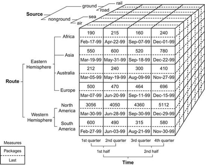
FIGURE 11.1 A (sources, routes, time) cube. Source: http://www.aspfree.com/c/a/MS-SQL-Server/Accessing-OLAP-using-ASP-dot-NET/

11.9.2 Dimensional Hierarchies

A listing of all of the cells in a hypercube is useless. We want to see aggregated (summary) information. We want to know that iPod sales are increasing, that we need to get rid of those bell-bottoms, that most of our business is in North America, and so forth.

Aggregation means that we need a hierarchy on the dimensions. Here is an example of a temporal dimension. Writing a hierarchy in SQL is easily done with a nested sets model if you have to write your own code:

CREATE TABLE TemporalDim

(range_name CHAR(15) NOT NULL PRIMARY KEY,

range_start_date DATE NOT NULL,

range_end_date DATE NOT NULL,

CHECK (range_start_date < range_end_date));

INSERT INTO TemporalDim

VALUES ('Year2006', '2006-01-01', '2006-12-31'),

('Qtr-01-2006', '2006-01-01', '2006-03-31'),

('Mon-01-2006', '2006-01-01', '2006-01-31'),

('Day:2006-01-01', '2006-01-01', '2006-01-01'),

..;

You can argue that you do not need to go to the leaf node level in the hierarchy, but only to the lowest level of aggregation. That will save space, but the code can be trickier when you have to show the leaf node level of the hierarchy.

This is the template for a hierarchical aggregation:

SELECT TD.range_name, ..

FROM TemporalDim AS TD, FactTable AS F

WHERE F.shipping_time BETWEEN TD.range_start_date

AND TD.range_end_date;

If you do not have the leaf nodes in the temporal dimension, then you need to add a CTE (common table expression) with the days and their names that are at the leaf nodes in your query:

WITH Calendar (date_name, cal_date)

AS VALUES (CAST ('2006-01-01' AS CHAR(15)),

CAST ('2006-01-01' AS DATE),

('2006-01-02', '2006-01-02'),

etc.

SELECT TD.range_name, ..

FROM Temporal_Dim AS TD, Fact_Table AS F

WHERE F.shipping_time BETWEEN TD.range_start_date

AND TD.range_end_date

UNION ALL

SELECT Calendar.date_name, ..

FROM Calendar AS C, FactTable AS F

WHERE C.cal_date = F.shipping_time;

A calendar table is used for other queries in the OLTP side of the house, so you should already have it in at least one database. You may also find that your cube tool automatically returns data at the leaf level if you ask it.

11.9.3 Drilling and Slicing

Many of the OLAP user interface tools will have a display with a dropdown menu for each dimension that lets you pick the level of aggregation in the report. The analogy is the slide switches on the front of expensive stereo equipment, which set how the music will be played, but not what songs are on the CD. It is called drilldown because you start at the highest level of the hierarchies and travel down the tree structure. Figure 11.2 is an example of such an interface from a Microsoft reporting tool.

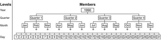
FIGURE 11.2 Example of a drilldown tree structure. Source: http://www.aspfree.com/c/a/MS-SQL-Server/Accessing-OLAP-using-ASP-dot-NET/

Slicing a cube is another physical analogy. Look at the illustration of the cube in Figure 11.1 and imagine that you have a cheese knife and you slice off blocks from the cube. For example, you might want to look at only the ground shipments, so you slice off just that dimension, building a subcube. The drilldowns will still be in place. This is like picking the song from a CD.

Concluding Thoughts

We invented a new occupation: data scientist! This does not have an official definition, but it seems to be a person who can use OLAP databases, statistics packages, and some of the NoSQL tools we have discussed. He or she also seems to need a degree in statistics or math. There have also been a lot of advances in statistics that use the improved, cheap computing power we have today. For example, the assumption of a normal distribution in data was made for convenience of computations for centuries. Today, we can use resampling, pareto, and exponential models, and even more complex math.

References

1. Codd EF. Providing OLAP to User-Analysts: An IT Mandate. Available at, http://www.minet.uni-jena.de/dbis/lehre/ss2005/sem_dwh/lit/Cod93.pdf; 1993.

2. Zemke F, Kulkarni K, Witkowski A, Lyle B. Introduction to OLAP functions (ISO/IEC JTC1/ SC32 WG3:YGJ-068 ANSI NCITS H2-99-154r2). 1999; In: ftp://ftp.iks-jena.de/mitarb/lutz/standards/sql/OLAP-99-154r2.pdf; 1999.