Expert Oracle SQL: Optimization, Deployment, and Statistics (2014)
PART 3. The Cost-Based Optimizer
CHAPTER 11. Joins
Every SQL query or subquery has a FROM clause that identifies one or more row sources. These row sources may be tables, data dictionary views, inline views, factored subqueries, or expressions involving the TABLE or XMLTABLE operators. If there is more than one row source then the rows produced by these row sources need to be joined, there being one less join operation than there are row sources. In Chapter 1 I covered the various different syntactic constructs for joins. These constructs included inner joins, left outer joins, right outer joins, full outer joins, and partitioned outer joins. I also explained which types of join could be constructed with traditional syntax and which required ANSI join syntax.
In this chapter I will look at the different methods that the runtime engine has for implementing joins of any type, the rules surrounding the order in which the row sources are joined, and how parallel execution can be used in joins. I will also look at two types of subquery unnesting: semi-joins and anti-joins. Subquery unnesting is an optimizer transformation for constructing additional row sources and joins that aren’t present in the FROM clause of the original query. But first let me review the four types of join method.
Join Methods
There are four methods that the runtime engine has at its disposal for implementing any join. These four methods are nested loops, hash join, merge join, and Cartesian join. The Cartesian join is just a simplified form of a merge join, so in a sense there are just three and a half join methods.
When an execution plan is displayed by DBMS_XPLAN the two operands of a join operation appear, one on top of the other, at the same level of indentation. In Chapter 1 I introduced the terms driving row source to refer to the top row source in the display and probe row source to refer to the bottom row source. As we shall shortly see, this terminology is appropriate for nested loops, merge joins, and Cartesian joins. To avoid confusion I will also refer to the top row source of a hash join as the driving row source and the bottom operand as the probe source, even though, as will be soon made clear, the terms aren’t entirely appropriate in the case of a hash join.
Chapter 1 also introduced some syntax for describing join orders. The syntax (T1 ![]() T2)
T2) ![]() T3 describes what I will refer to as a join tree involving two joins. The first join to occur is between T1 and T2, with T1 being the driving row source and T2 being the probe row source. This join creates an intermediate result set that becomes the driving row source of a second join operation, with T3 as the probe row source. I will continue to use the same terminology throughout this chapter. Let us now look at the first of the four join methods, nested loops.
T3 describes what I will refer to as a join tree involving two joins. The first join to occur is between T1 and T2, with T1 being the driving row source and T2 being the probe row source. This join creates an intermediate result set that becomes the driving row source of a second join operation, with T3 as the probe row source. I will continue to use the same terminology throughout this chapter. Let us now look at the first of the four join methods, nested loops.
Nested loops
The nested loops join method, and only the nested loops join method, can be used to support correlated row sources by means of a left lateral join. I will address left lateral joins shortly, but let me first look at what I will refer to as traditional nested loops, which implement joins between uncorrelated row sources.
Traditional nested loops
Listing 11-1 joins the two most famous Oracle database tables from the most famous example database schema.
Listing 11-1. Joining EMP and DEPT using nested loops (10.2.0.5)
SELECT /*+
gather_plan_statistics
optimizer_features_enable('10.2.0.5')
leading(e)
use_nl(d)
index(d)
*/
e.*, d.loc
FROM scott.emp e, scott.dept d
WHERE hiredate > DATE '1980-12-17' AND e.deptno = d.deptno;
SET LINES 200 PAGES 0
SELECT * FROM TABLE (DBMS_XPLAN.display_cursor (format=>
'BASIC +IOSTATS LAST -BYTES -ROWS +PREDICATE'));
------------------------------------------------------------------
| Id | Operation | Name | Starts | A-Rows |
------------------------------------------------------------------
| 0 | SELECT STATEMENT | | 1 | 13 |
| 1 | NESTED LOOPS | | 1 | 13 | -- Extra columns
|* 2 | TABLE ACCESS FULL | EMP | 1 | 13 | -- removed
| 3 | TABLE ACCESS BY INDEX ROWID| DEPT | 13 | 13 |
|* 4 | INDEX UNIQUE SCAN | PK_DEPT | 13 | 13 |
------------------------------------------------------------------
Predicate Information (identified by operation id):
---------------------------------------------------
2 - filter("HIREDATE">TO_DATE(' 1980-12-17 00:00:00', 'syyyy-mm-dd
hh24:mi:ss'))
4 - access("E"."DEPTNO"="D"."DEPTNO")
Listing 11-1 joins the EMP and DEPT tables from the example SCOTT schema. I have once again used hints to generate the execution plan I want to discuss, as the CBO would have picked a more efficient plan otherwise. I have used the LEADING hint to specify that the driving row source is the EMP table and an INDEX hint so that DEPT is accessed by an index. So that I can explain different aspects of nested loops in stages, I have also used the OPTIMIZER_FEATURES_ENABLE hint so that the 10.2.0.5 implementation is used. The GATHER_PLAN_STATISTICShint is used to get runtime data from DBMS_XPLAN.DISPLAY_CURSOR.
The NESTED LOOPS operation on line 1 begins by accessing the driving table EMP. The semantics of an inner join mean that logically all predicates in the WHERE clause are processed after the join operation. However, in reality the predicate hiredate > DATE '1980-12-17' is specific to the EMP table and the CBO eliminates any row that doesn’t match this filter condition as soon as possible, as is confirmed by the predicate section of the execution plan in Listing 11-1 that shows the filter being applied by operation 2. As each of the 13 rows in EMP with a suitable hiring date are found, the rows from DEPT matching the join predicate e.deptno = d.deptno are identified and returned.
Although three matching rows in EMP have a DEPTNO of 10, five have a DEPTNO of 20, and five of the thirteen rows have a value of 30 for DEPTNO, it is still possible to use an index on DEPT.DEPTNO. The pseudo-code looks something like this:
For each row in EMP subset
LOOP
For each matching row in DEPT
LOOP
<return row>
END LOOP
END LOOP
Hence the term nested loops. You can see from the STARTS column of the DBMS_XPLAN.DISPLAY_CURSOR results that the index lookup on PK_DEPT on line 4 and the DEPT table access on line 3 have been performed 13 times, once for each matching row from EMP.
![]() Tip The STARTS column for the probe row source of a nested loops operation usually matches the A-ROWS columns for the driving row source. This same tip applies to the LAST_STARTS and LAST_OUTPUT_ROWS in V$STATISTICS_PLAN_ALL. Semi-joins and anti-joins are exceptions to this rule as these take advantage of scalar subquery caching. I will cover semi-joins and anti-joins shortly.
Tip The STARTS column for the probe row source of a nested loops operation usually matches the A-ROWS columns for the driving row source. This same tip applies to the LAST_STARTS and LAST_OUTPUT_ROWS in V$STATISTICS_PLAN_ALL. Semi-joins and anti-joins are exceptions to this rule as these take advantage of scalar subquery caching. I will cover semi-joins and anti-joins shortly.
Listing 11-2 lets us see what happens when we change the OPTIMIZER_FEATURES_ENABLE hint to enable some 11gR1 functionality.
Listing 11-2. Joining EMP and DEPT using a nested loop (11.2.0.1)
SELECT /*+
gather_plan_statistics
optimizer_features_enable('11.2.0.1')
leading(e)
use_nl(d)
index(d)
no_nlj_batching(d)
*/
e.*, d.loc
FROM scott.emp e, scott.dept d
WHERE hiredate > DATE '1980-12-17' AND e.deptno = d.deptno;
SET LINES 200 PAGES 0
SELECT * FROM TABLE (DBMS_XPLAN.display_cursor (format=>
'BASIC +IOSTATS LAST -BYTES -ROWS +PREDICATE'));
--------------------------------------------------------------------------
| Id | Operation | Name | Starts | E-Rows | A-Rows |
--------------------------------------------------------------------------
| 0 | SELECT STATEMENT | | 0 | | 0 |
| 1 | TABLE ACCESS BY INDEX ROWID| DEPT | 1 | 1 | 13 |
| 2 | NESTED LOOPS | | 1 | 13 | 27 |
|* 3 | TABLE ACCESS FULL | EMP | 1 | 13 | 13 |
|* 4 | INDEX UNIQUE SCAN | PK_DEPT | 13 | 1 | 13 |
--------------------------------------------------------------------------
Predicate Information (identified by operation id):
---------------------------------------------------
3 - filter("HIREDATE">TO_DATE(' 1980-12-17 00:00:00', 'syyyy-mm-dd hh24:mi:ss'))
4 - access("E"."DEPTNO"="D"."DEPTNO")
In addition to the change in the OPTIMIZER_FEATURES_ENABLE parameter, Listing 11-2 also disables one of the new features of 11gR1 by using the NO_NLJ_BATCHING hint. The execution plan in Listing 11-2 differs from that in Listing 11-1 in that the join operation is a child of operation 1—the TABLE ACCESS BY INDEX ROWID. This approach is called nested loop prefetching and was available in 9i for an INDEX RANGE SCAN, but only became available for an INDEX UNIQUE SCAN in 11gR1. Nested loop prefetching allows operation 1 to obtain a number of ROWIDs from its child operation on line 2 before deciding what to do next. In the case where the returned ROWIDs are in consecutive blocks, none of which are in the buffer cache, operation 1 can gain some performance by making a single multi-block read in lieu of multiple single-block reads. Notice that in Listing 11-1 the TABLE ACCESS BY INDEX ROWID operation on line 3 shows a value of 13 in the STARTS column, as opposed to operation 1 in Listing 11-2, which shows a value of 1. In the latter case one invocation of operation 1 is sufficient as all the ROWIDs are obtained from the child on line 2.
Listing 11-3 shows what happens when we remove the two hints in bold from Listing 11-2.
Listing 11-3. Nested loops join batching
SELECT /*+
gather_plan_statistics
leading(e)
use_nl(d)
index(d)
*/
e.*, d.loc
FROM scott.emp e, scott.dept d
WHERE hiredate > DATE '1980-12-17' AND e.deptno = d.deptno;
SET LINES 200 PAGES 0
SELECT *
FROM TABLE (
DBMS_XPLAN.display_cursor (
format => 'BASIC +IOSTATS LAST -BYTES +PREDICATE'));
---------------------------------------------------------------------------
| Id | Operation | Name | Starts | E-Rows | A-Rows |
---------------------------------------------------------------------------
| 0 | SELECT STATEMENT | | 1 | | 13 |
| 1 | NESTED LOOPS | | 1 | | 13 |
| 2 | NESTED LOOPS | | 1 | 13 | 13 |
|* 3 | TABLE ACCESS FULL | EMP | 1 | 13 | 13 |
|* 4 | INDEX UNIQUE SCAN | PK_DEPT | 13 | 1 | 13 |
| 5 | TABLE ACCESS BY INDEX ROWID| DEPT | 13 | 1 | 13 |
---------------------------------------------------------------------------
Here we have employed an optimization known as nested loop batching. We now have two NESTED LOOPS operations for one join. Although nested loop batching is not officially an optimizer transformation, the CBO has effectively transformed the original query into that shown inListing 11-4.
Listing 11-4. Simulating 11g nested loops in 10g
SELECT /*+ leading(e d1)
use_nl(d)
index(d)
rowid(d)
optimizer_features_enable('10.2.0.5') */
e.*, d.loc
FROM scott.emp e, scott.dept d1, scott.dept d
WHERE e.hiredate > DATE '1980-12-17'
AND e.deptno = d1.deptno
AND d.ROWID = d1.ROWID;
-----------------------------------------------
| Id | Operation | Name |
-----------------------------------------------
| 0 | SELECT STATEMENT | |
| 1 | NESTED LOOPS | |
| 2 | NESTED LOOPS | |
| 3 | TABLE ACCESS FULL | EMP |
| 4 | INDEX UNIQUE SCAN | PK_DEPT |
| 5 | TABLE ACCESS BY USER ROWID| DEPT |
-----------------------------------------------
The execution plan in Listing 11-4 is remarkably similar to that in Listing 11-3 even though the OPTIMIZER_FEATURES_ENABLE hint disables all 11g features. The query in Listing 11-4 includes two copies of DEPT and one copy of EMP, making three row sources in total, and, therefore, two joins are necessary. The one difference between the execution plans in Listings 12-3 and 12-4 is that since we have specified ROWIDs ourselves in Listing 11-4 the access to the table is by means of a TABLE ACCESS BY USER ROWID operation rather than by the TABLE ACCESS BY INDEX ROWID operation in Listing 11-3.
The performance benefits of nested loop batching are not obvious from the DBMS_XPLAN display: the STARTS column for operations 4 and 5 in Listing 11-3 still shows 13 probes for 13 rows, but in some cases physical and logical I/O operations may be reduced nonetheless.
![]() Tip You will notice in Listing 11-3 see that the E-ROWS column (estimated rows) for operations 4 and 5 of the execution plan shows a value of 1 and the A-ROWS column (actual rows) shows a value of 13. This is not a cardinality error by the CBO. In the case of NESTED LOOPS the estimated row count is per iteration of the loop whereas the actual row count is for all iterations of the loop.
Tip You will notice in Listing 11-3 see that the E-ROWS column (estimated rows) for operations 4 and 5 of the execution plan shows a value of 1 and the A-ROWS column (actual rows) shows a value of 13. This is not a cardinality error by the CBO. In the case of NESTED LOOPS the estimated row count is per iteration of the loop whereas the actual row count is for all iterations of the loop.
Nested loops have the desirable property that they usually scale linearly. By that I mean that if EMP and DEPT double in size the nested loop will take twice as much time (as opposed to much more).
However, nested loops have two undesirable performance properties:
· Unless the probe table is part of a hash cluster (oops! I said I wouldn’t mention hash clusters again) or is very small, an index is required on the joined column or columns, in this case DEPT.DEPTNO. If such an index is not present then we might need to visit every row in DEPT for every row in EMP. Not only is this often very costly in itself, it also wrecks the scalability property of the join: if we double the size of EMP and DEPT then the loop takes four times as long because we access DEPT twice as often, because EMP is twice as big, and each scan takes twice as long, because DEPT is twice as big. Note that indexing is usually not possible if the probe row source of the nested loop is a subquery or inline view. For this reason, when joining a table and a subquery or inline view using nested loops, the probe row source will almost always be the table.
· When the probe row source is a table, blocks in the probed table may be visited many times, picking out different rows each time.
Left Lateral Joins
Prior to release 12cR1, a left lateral join was only available in conjunction with the TABLE and XMLTABLE operators that we covered in Chapter 10. I have showed an example of a join involving DBMS_XPLAN.DISPLAY in Listing 8-9. In release 12cR1 this useful feature has become more accessible by means of the LATERAL keyword. Listing 11-5 shows an example of its use.
Listing 11-5. Left lateral join
SELECT e1.*, e3.avg_sal
FROM scott.emp e1
,LATERAL (SELECT AVG (e2.sal) avg_sal
FROM scott.emp e2
WHERE e1.deptno != e2.deptno) e3;
------------------------------------------------
| Id | Operation | Name |
------------------------------------------------
| 0 | SELECT STATEMENT | |
| 1 | NESTED LOOPS | |
| 2 | TABLE ACCESS FULL | EMP |
| 3 | VIEW | VW_LAT_A18161FF |
| 4 | SORT AGGREGATE | |
|* 5 | TABLE ACCESS FULL| EMP |
------------------------------------------------
Predicate Information (identified by operation id):
---------------------------------------------------
5 - filter("E1"."DEPTNO"<>"E2"."DEPTNO")
Listing 11-5 lists the details of each employee together with the average salaries of all employees in departments other than that in which the employee in question works.
A left lateral join is always implemented by nested loops, and the inline view preceded by LATERAL is always the probe row source. The key advantage of lateral joins is that predicates can be used in the inline view derived from columns in the driving row source. I will use lateral joins to great effect when I look at optimizing sorts in Chapter 17.
It is possible to perform an outer lateral join by placing the characters (+) after the inline view, but as I explained in Chapter 1 I prefer to use ANSI syntax for outer joins. ANSI syntax uses the keywords CROSS APPLY for an inner lateral join and OUTER APPLY for an outer lateral join; I will provide examples of both variants when I cover optimizer transformations in Chapter 13.
Hash joins
There are two variants of the hash join depending on whether join inputs are swapped or not. Let us discuss the standard hash join without join input swapping first and then consider the variation in which join inputs are swapped as part of a wider discussion of join orders a little later in this chapter.
Let us begin by looking at Listing 11-6, which changes the hints in Listing 11-3 to specify a hash join rather than a nested loop.
Listing 11-6. Hash join
SELECT /*+ gather_plan_statistics
leading(e)
use_hash(d)
*/
e.*, d.loc
FROM scott.emp e, scott.dept d
WHERE hiredate > DATE '1980-12-17' AND e.deptno = d.deptno;
SELECT *
FROM TABLE (DBMS_XPLAN.display_cursor (format => 'BASIC +IOSTATS LAST'));
--------------------------------------------------------------
| Id | Operation | Name | Starts | E-Rows | A-Rows |
--------------------------------------------------------------
| 0 | SELECT STATEMENT | | 1 | | 13 |
|* 1 | HASH JOIN | | 1 | 13 | 13 |
|* 2 | TABLE ACCESS FULL| EMP | 1 | 13 | 13 |
| 3 | TABLE ACCESS FULL| DEPT | 1 | 4 | 4 |
--------------------------------------------------------------
Predicate Information (identified by operation id):
---------------------------------------------------
1 - access("E"."DEPTNO"="D"."DEPTNO")
2 - filter("HIREDATE">TO_DATE(' 1980-12-17 00:00:00', 'syyyy-mm-dd
hh24:mi:ss'))
The hash join operates by placing the 13 rows from EMP that match the selection predicate into a workarea containing an in-memory hash cluster keyed on EMP.DEPTNO. The hash join then makes a single pass through the probe table DEPT, and for each row we apply the hash toD.DEPTNO and find any matching rows in EMP.
In this regard the hash join is similar to a nested loops join, with DEPT as the driving row source and the copy of the EMP table stored in the in-memory hash cluster as the probe row source. Nevertheless, for consistency I will continue to refer to EMP as the driving row source in our join. Hash joins have the following advantages over nested loops when the probe row source is a table:
· Every block in the probe table is visited at most once and not potentially multiple times as with a nested loop.
· No index is required on the join column in the probe table.
· If a full table scan (or fast full index scan) is used for accessing the probe table then multi-block reads can be used, which are much more efficient than single-block reads through an index.
· Join inputs can be swapped. We will discuss hash join input swapping very shortly.
However, hash joins have the following disadvantages:
· If a block in the probe table contains no rows that match any of the rows in the driving row source it may still be visited. So, for example, if the size of the probe table was 1TB, there was no selection predicate, and only two rows matched the join predicates, we would scan the whole 1TB table rather than picking out two rows through an index.
· While both join operands are small, hash joins scale linearly as nested loops do. However, if the driving row source gets too big the hash table will spill onto disk, ruining the linear performance properties.
· Hash joins can only be used with equality join predicates.
When an index is available on the probe row source it may be that a nested loops join will visit some blocks multiple times and some not at all. Deciding between the nested loops join with an index and the hash join that visits all blocks exactly once via a full table scan can be difficult. The optimizer uses the selectivity of the join predicate in conjunction with the clustering factor of the index to help determine the correct course of action, as we discussed in Chapter 9.
Merge joins
A merge join is very similar to a merge sort. Both the driving and probe row sources are sorted to start with and placed into process-private workareas. We then proceed in a way similar to that for a nested loops join: for each row in the driving row source we look for all the rows in the probe row source that match that one row in the driving row source. In the case of an equality join predicate such as T1.C1=T2.C2 we can proceed through the two sorted sets in step. However, merge joins can also take advantage of range-based join predicates, such as T1.C1 < T2.C2. In this case, we may need to “backup” the point at which we examine the sorted probe row source as we advance through the driving row source.
Consider Listing 11-7, which includes a range-based join predicate.
Listing 11-7. Query containing a range-based join predicate
CREATE TABLE t1
AS
SELECT ROWNUM c1
FROM all_objects
WHERE ROWNUM <= 100;
CREATE TABLE t2
AS
SELECT c1 + 1 c2 FROM t1;
CREATE TABLE t3
AS
SELECT c2 + 1 c3 FROM t2;
CREATE TABLE t4
AS
SELECT c3 + 1 c4 FROM t3;
SELECT /*+ leading (t1) use_merge(t2)*/
*
FROM t1, t2
WHERE t1.c1 > 3 AND t2.c2 < t1.c1;
------------------------------------
| Id | Operation | Name |
------------------------------------
| 0 | SELECT STATEMENT | |
| 1 | MERGE JOIN | |
| 2 | SORT JOIN | |
| 3 | TABLE ACCESS FULL| T1 |
| 4 | SORT JOIN | |
| 5 | TABLE ACCESS FULL| T2 |
------------------------------------
Figure 11-1 shows how a merge join driven by T1 would be implemented:
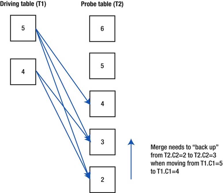
Figure 11-1. A merge join
Notice how:
· Both T1 and T2 have been sorted in descending order because of the "<" predicate. If the predicate were "=", ">", or ">=" both tables would have been sorted in ascending order.
· Because of the selection predicate the workarea for T1 only contains two rows.
Merge joins are a relatively rare choice of join mechanism these days but can be useful under one or more of the following conditions:
· The first row source is already sorted, avoiding the need for the first of the two sorts normally performed by the merge join. Be aware that the second row source is always sorted even if it is sorted to start with!
· The row sources are required to be sorted by the join column (for example, because of an ORDER BY clause). As the results of the join are generated ready-sorted, the extra step is avoided.
· There is no index on the joined columns and/or the selectivity/clustering factor is weak (making nested loops unattractive).
· The join predicate is a range predicate (ruling out hash joins).
· Both row sources being joined are so large that neither can be hashed into memory (making hash joins unattractive). Be aware that merge joins can also spill onto disk, but the impact may not be as bad as for hash joins that spill onto disk.
Cartesian joins
Cartesian joins are very similar to merge joins (they appear as MERGE JOIN CARTESIAN in the execution plan). This is the join method of last resort and is almost only used when there is no join predicate available (unless you use the undocumented and probably uselessUSE_MERGE_CARTESIAN hint). This join method operates just like a merge join except that as every row in the driving row source matches every row in the probe row source no sorts take place. It may seem like one sort occurs because you will see a BUFFER SORT operation in the execution plan but this is misleading. There is buffering but no sorting. If there are m rows in the driving row source and n rows in the probe row source then there will be m x n rows returned by the join. Cartesian joins should not be a performance concern provided that m x n is small and/or either m or n is zero. Listing 11-8 shows a Cartesian join.
Listing 11-8. Cartesian join
SELECT /*+ leading (t1) use_merge_cartesian(t2)*/
*
FROM t1, t2;
-------------------------------------
| Id | Operation | Name |
-------------------------------------
| 0 | SELECT STATEMENT | |
| 1 | MERGE JOIN CARTESIAN| |
| 2 | TABLE ACCESS FULL | T1 |
| 3 | BUFFER SORT | |
| 4 | TABLE ACCESS FULL | T2 |
-------------------------------------
Just to repeat, the BUFFER SORT operation buffers but does not sort.
Join Orders
Hash join input swapping is a mechanism for generating additional join orders that wouldn’t otherwise be available to the CBO. However, before we get into hash join input swapping let us make sure we understand the legal join orders available without hash join input swapping first.
Join orders without hash join input swapping
Prior to the implementation of hash join input swapping the following restrictions on join order applied:
· The first join would have been between two row sources from the FROM clause generating an intermediate result set.
· The second and all subsequent joins would use the intermediate result set from the preceding join as the driving row source and a row source from the FROM clause as the probe row source.
Let me provide an example. If we join the four tables we created in Listing 1-18, T1, T2, T3, and T4, with inner joins, then one possible join tree is ((T1 ![]() T2)
T2) ![]() T3)
T3) ![]() T4. You can shuffle the tables around. You have four choices for the first table, three for the second, two for the third, and one for the fourth, generating 24 possible legal join orders. This type of join ordering results in what is known as a left-deep join tree. The reason for the term is clear if we draw the joins in a diagram as in Figure 11-2.
T4. You can shuffle the tables around. You have four choices for the first table, three for the second, two for the third, and one for the fourth, generating 24 possible legal join orders. This type of join ordering results in what is known as a left-deep join tree. The reason for the term is clear if we draw the joins in a diagram as in Figure 11-2.
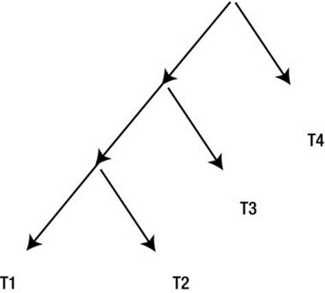
Figure 11-2. Left-deep join tree
Figure 11-2 shows arrows pointing downwards because the join operations invoke their children to access the tables. However, you might prefer to draw the arrows pointing upwards; doing so would reflect how the data flows.
The left-deep join tree leads to a simple set of optimizer hints for specifying join order and join method:
· The LEADING hint specifies the first few (or all) row sources in the join. For example, LEADING(T1 T2) forces the CBO to join T1 and T2 to start with. T1 must be the driving row source and T2 the probe row source. Whether T3 or T4 is joined next is up to the CBO.
· The hints USE_NL, USE_HASH, USE_MERGE, and USE_MERGE_CARTESIAN specify join methods. To identify which join the hint refers to, we use the name of the probe row source.
This is all a bit abstract, but hopefully the example in Listing 11-9 will make things clear.
Listing 11-9. Fully specifying join orders and join methods
SELECT /*+
leading (t4 t3 t2 t1)
use_nl(t3)
use_nl(t2)
use_nl(t1)
*/
*
FROM t1
,t2
,t3
,t4
WHERE t1.c1 = t2.c2 AND t2.c2 = t3.c3 AND t3.c3 = t4.c4;
-------------------------------------
| Id | Operation | Name |
-------------------------------------
| 0 | SELECT STATEMENT | |
| 1 | NESTED LOOPS | |
| 2 | NESTED LOOPS | |
| 3 | NESTED LOOPS | |
| 4 | TABLE ACCESS FULL| T4 |
| 5 | TABLE ACCESS FULL| T3 |
| 6 | TABLE ACCESS FULL | T2 |
| 7 | TABLE ACCESS FULL | T1 |
-------------------------------------
The LEADING hint in Listing 11-9 has specified all the tables, so the join order is fixed as ((T4 ![]() T3)
T3) ![]() T2)
T2) ![]() T1. When hinting the join mechanisms, the three joins are identified by their respective probe row sources: T3, T2, and T1. In this case a hint specifying T4 would be meaningless as it is not the probe row source in any join.
T1. When hinting the join mechanisms, the three joins are identified by their respective probe row sources: T3, T2, and T1. In this case a hint specifying T4 would be meaningless as it is not the probe row source in any join.
Join orders with hash join input swapping
In the case of hash joins, and hash joins only, the optimizer can swap the inputs to a join without the need for inline views. So, for example, suppose we started out with a join order ((T1 ![]() T2)
T2) ![]() T3)
T3) ![]() T4 and we swapped the inputs to the final join with T4. We end up with T4
T4 and we swapped the inputs to the final join with T4. We end up with T4 ![]() ((T1
((T1 ![]() T2)
T2) ![]() T3). We now have, for the first time, a join with a probe row source that is an intermediate result set. Let us continue the process and swap the join inputs for the second join with T3. This yields T4
T3). We now have, for the first time, a join with a probe row source that is an intermediate result set. Let us continue the process and swap the join inputs for the second join with T3. This yields T4 ![]() (T3
(T3 ![]() (T1
(T1 ![]() T2)). We also have the option of swapping the join with T2. The result of swapping the join inputs of the join of T1 and T2 is (T4
T2)). We also have the option of swapping the join with T2. The result of swapping the join inputs of the join of T1 and T2 is (T4 ![]() (T3
(T3 ![]() (T2
(T2 ![]() T1))). Swapping the join inputs of the join of T1 and T2 seems pointless: we could just change the join order instead. But let us not get distracted. I’ll soon show you why swapping the join inputs of the first join might be useful. Listing 11-10 shows how we might hint the query in Listing 11-9 in different ways to control join input swapping.
T1))). Swapping the join inputs of the join of T1 and T2 seems pointless: we could just change the join order instead. But let us not get distracted. I’ll soon show you why swapping the join inputs of the first join might be useful. Listing 11-10 shows how we might hint the query in Listing 11-9 in different ways to control join input swapping.
Listing 11-10. A simple example comparing swapped and unswapped join inputs
SELECT /*+ SELECT /*+
leading (t1 t2 t3 t4) leading (t1 t2 t3 t4)
use_hash(t2) use_hash(t2)
use_hash(t3) use_hash(t3)
use_hash(t4) use_hash(t4)
no_swap_join_inputs(t2) swap_join_inputs(t2)
no_swap_join_inputs(t3) swap_join_inputs(t3)
no_swap_join_inputs(t4) swap_join_inputs(t4)
*/ */
* *
FROM t1 FROM t1
,t2 ,t2
,t3 ,t3
,t4 ,t4
WHERE t1.c1 = t2.c2 WHERE t1.c1 = t2.c2
AND t2.c2 = t3.c3 AND t2.c2 = t3.c3
AND t3.c3 = t4.c4; AND t3.c3 = t4.c4;
---------------------------------------- --------------------------------------
| Id | Operation | Name | | Id | Operation | Name |
---------------------------------------- --------------------------------------
| 0 | SELECT STATEMENT | | | 0 | SELECT STATEMENT | |
| 1 | HASH JOIN | | | 1 | HASH JOIN | |
| 2 | |HASH JOIN | | | 2 | |TABLE ACCESS FULL | T4 |
| 3 | | |HASH JOIN | | | 3 | |HASH JOIN | |
| 4 | | | |TABLE ACCESS FULL| T1 | | 4 | |TABLE ACCESS FULL | T3 |
| 5 | | | |TABLE ACCESS FULL| T2 | | 5 | |HASH JOIN | |
| 6 | | |TABLE ACCESS FULL | T3 | | 6 | |TABLE ACCESS FULL| T2 |
| 7 | |TABLE ACCESS FULL | T4 | | 7 | |TABLE ACCESS FULL| T1 |
---------------------------------------- --------------------------------------
The left-hand side of Listing 11-10 shows the traditional left-deep join tree with none of the join inputs swapped. This has been enforced with the use of NO_SWAP_JOIN_INPUTS hints. You will notice that the intermediate result set from the join on line 3 is used as the driving row source of the join on line 2 (line 3 is vertically above line 6) and that the intermediate result set of the join on line 2 is the driving row source of the join on line 1 (line 2 is vertically above line 7). I have added some lines to the DBMS_XPLAN output in order to make the alignment clear.
On the other hand, the right-hand side of Listing 11-10 swaps all join inputs by means of SWAP_JOIN_INPUTS hints. Now you can see that the intermediate result set formed by the join on line 5 is the probe row source of the join on line 3 (line 5 is vertically below line 4), and the intermediate result set formed by the join on line 3 is the probe row source of the join on line 1 (line 3 is vertically below line 2). The result of swapping all join inputs is referred to as a right-deep join tree and is depicted pictorially by Figure 11-3.
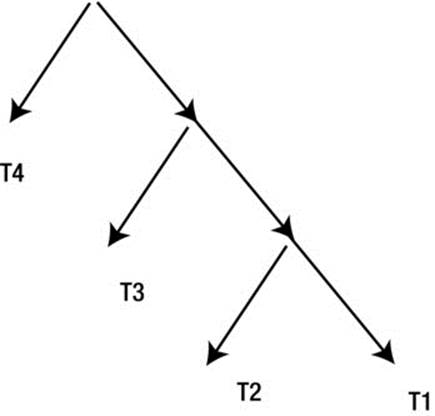
Figure 11-3. Right-deep join tree
![]() Note If some joins in a query have their inputs swapped and others do not then the resulting join tree is referred to as a zigzag tree. Join trees such as (T1
Note If some joins in a query have their inputs swapped and others do not then the resulting join tree is referred to as a zigzag tree. Join trees such as (T1 ![]() T2)
T2) ![]() (T3
(T3 ![]() T4) are referred to as bushy joins, but bushy joins are never considered by the CBO.
T4) are referred to as bushy joins, but bushy joins are never considered by the CBO.
Now that the CBO has created this right-deep join tree, what does the runtime engine do with it? Well, despite the LEADING hint claiming that we start with table T1, the runtime engine actually begins by placing the selected rows from T4 into an in-memory hash cluster in a workarea. It then places the contents of T3 into a second workarea and T2 into a third. What then happens is that T1 is scanned and rows from T1 are matched with T2. The results of any matches of T1 and T2 are matched with rows from T3. Finally, the matching rows from the joins of T1, T2, and T3are matched against the rows from T4.
The benefits of a right-deep join tree may not be immediately apparent. At first glance a left-deep join tree seems more memory efficient than a right-deep join tree. The runtime engine begins processing the join operation on line 3 in the left-deep join tree in Listing 11-10 by placing T1into a workarea. As T2 is scanned and matches are found, the joined rows are placed into a second workarea associated with the join on line 2. At the conclusion of the scan of T2 the workarea containing T1 is no longer required and is dropped before the new workarea needed by operation 1 to receive the results of the join with T3 is created. So a left-deep join tree only ever has two workareas. On the other hand, a right-deep join tree with n joins requires n concurrent workareas.
The best way to understand the benefits of right-deep join trees is to look at an example from data warehousing. Listing 11-11 uses tables from the SH example schema.
Listing 11-11. Swapped hash join inputs in a data warehousing environment
SELECT * SELECT /*+
FROM sh.sales leading (sales customers products)
JOIN sh.products use_hash(customers)
USING (prod_id) use_hash(products)
LEFT JOIN sh.customers no_swap_join_inputs(customers)
USING (cust_id); swap_join_inputs(products)
*/ *
FROM sh.sales
JOIN sh.products USING (prod_id)
LEFT JOIN sh.customers USING (cust_id);
------------------------------------------ -----------------------------------------
| Id| Operation | Name | | Id| Operation | Name |
------------------------------------------ -----------------------------------------
| 0 | SELECT STATEMENT | | | 0 | SELECT STATEMENT | |
| 1 | HASH JOIN | | | 1 | HASH JOIN | |
| 2 | TABLE ACCESS FULL | PRODUCTS | | 2 | TABLE ACCESS FULL | PRODUCTS |
| 3 | HASH JOIN RIGHT OUTER| | | 3 | HASH JOIN OUTER | |
| 4 | TABLE ACCESS FULL | CUSTOMERS | | 4 | PARTITION RANGE ALL| |
| 5 | PARTITION RANGE ALL | | | 5 | TABLE ACCESS FULL | SALES |
| 6 | TABLE ACCESS FULL | SALES | | 6 | TABLE ACCESS FULL | CUSTOMERS |
------------------------------------------ -----------------------------------------
Listing 11-11 joins the SALES table with the CUSTOMERS and PRODUCTS tables, both with and without hints. The actual SALES data always specifies a customer for each sale, but for demonstration purposes I want to protect against the possibility that the CUST_ID field in the SALEStable may be NULL, so I will use an outer join to ensure rows in SALES are not lost.
The biggest table in Listing 2-9 is SALES, with 918,843 rows, and so we would like to read that table last to avoid building a huge hash cluster that may not fit into memory. The PRODUCTS table has 72 rows and the CUSTOMERS table has 55,500 rows, but, unfortunately, there is no predicate on which to join the PRODUCTS and CUSTOMERS tables, and the result of joining them with a Cartesian join would be to yield an intermediate result with 3,996,000 rows (72 x 55,500). Let us see how the CBO addresses the problem.
If you look closely you will see that the join order from the unhinted query is PRODUCTS ![]() (CUSTOMERS
(CUSTOMERS ![]() SALES)—a right-deep join tree. Rather than joining PRODUCTS and CUSTOMERS with a Cartesian join, generating one huge workarea, we have created one workarea with 72 rows and another workarea with 55,500 rows. The SALES table is then scanned once, and the query returns rows from SALES that match both the CUSTOMERS and PRODUCTS tables. So that’s the answer. Right-deep join trees can be used when joining one big table with multiple small tables by creating multiple small workareas rather than one or more big ones.
SALES)—a right-deep join tree. Rather than joining PRODUCTS and CUSTOMERS with a Cartesian join, generating one huge workarea, we have created one workarea with 72 rows and another workarea with 55,500 rows. The SALES table is then scanned once, and the query returns rows from SALES that match both the CUSTOMERS and PRODUCTS tables. So that’s the answer. Right-deep join trees can be used when joining one big table with multiple small tables by creating multiple small workareas rather than one or more big ones.
There is one more interesting observation to make about the unhinted execution plan in Listing 11-11: the preserved row source in the outer join on line 3 is the probe row source.
The HASH JOIN RIGHT OUTER operation in Listing 11-11 works as follows:
· Rows from CUSTOMERS table are placed into a hash cluster.
· All the partitions of SALES are scanned. Each row from SALES is matched against CUSTOMERS and any matches are passed to the join with PRODUCTS.
· If there are no matches in CUSTOMERS for a row from SALES then the row from SALES is still passed up to the join with PRODUCTS.
The right-hand side of Listing 11-11 uses hints to suppress the swapping of the inputs of the SALES and CUSTOMERS tables but is otherwise identical to the left-hand side. The HASH JOIN OUTER operation works in a completely different way:
· The SALES table is placed into the in-memory hash cluster (not good for performance on this occasion).
· The CUSTOMERS table is scanned and any matches found in SALES are passed up to the join with PRODUCTS.
· When matches are found, the entries in the SALES in-memory hash cluster are marked.
· At the end of the scan of CUSTOMERS any entries from the SALES hash cluster that have not been marked are passed to the join with PRODUCTS.
OUTER JOIN OPERATIONS
There are a number of operations that support different flavors of outer join. These include NESTED LOOPS OUTER, HASH JOIN OUTER, HASH JOIN RIGHT OUTER, HASH JOIN FULL OUTER, MERGE JOIN OUTER, and MERGE JOIN PARTITION OUTER.
· Only the hash join mechanism directly supports full outer joins.
· For some reason the first operand of a HASH JOIN FULL OUTER operation has to be the row source written to the left of the word FULL, but the join inputs can be swapped.
· You cannot get a HASH JOIN RIGHT OUTER operation by changing the join order. You need to swap join inputs.
· With the exception of the HASH JOIN RIGHT OUTER operation, the driving row source is preserved and the probe row source is optional.
· Only nested loops and merge joins support partitioned outer joins.
Although we have now covered the implementation of all explicitly written join operations, the CBO can generate additional joins that aren't written as such. Let us move on to semi-joins, the first of the two types of joins that the CBO can fabricate.
Semi-joins
It turns out that the optimizer can transform some constructs that you don’t write as joins into joins. We will begin by looking at semi-joins and then move on to anti-joins. There are two types of semi-join: standard and null-accepting semi-joins. Let us look at standard semi-joins first.
Standard semi-joins
Consider Listing 11-12, which looks for countries that have customers:
Listing 11-12. Semi-join
SELECT * SELECT *
FROM sh.countries FROM sh.countries
WHERE country_id IN (SELECT WHERE country_id IN (SELECT /*+ NO_UNNEST */
country_id FROM sh.customers); country_id FROM sh.customers);
-------------------------------------- --------------------------------------
| Id| Operation | Name | | Id| Operation | Name |
-------------------------------------- --------------------------------------
| 0 | SELECT STATEMENT | | | 0 | SELECT STATEMENT | |
| 1 | HASH JOIN SEMI | | | 1 | FILTER | |
| 2 | TABLE ACCESS FULL| COUNTRIES | | 2 | TABLE ACCESS FULL| COUNTRIES |
| 3 | TABLE ACCESS FULL| CUSTOMERS | | 3 | TABLE ACCESS FULL| CUSTOMERS |
-------------------------------------- --------------------------------------
When the runtime engine runs the execution plan on the left-hand side of Listing 11-12, it begins by creating an in-memory hash cluster of COUNTRIES as with a normal hash join and then processes the CUSTOMERS looking for a match. However, when the runtime engine finds a match, it removes the entry from the in-memory hash cluster so that the same country isn’t returned again.
The process of changing a subquery into a join is called subquery unnesting and is an example of an optimizer transformation. We will speak more about optimizer transformations in Chapter 13, but this is a sneak preview. Like all optimizer transformations, subquery unnesting is controlled by two hints. The UNNEST hint wasn’t required on the left-hand side, as the CBO chose the transformation itself. The transformation was explicitly suppressed on the right-hand side of Listing 11-12 by means of a NO_UNNEST hint. Without the aid of subquery unnesting theCUSTOMERS table is scanned 23 times, once for each row in COUNTRIES.
Nested loops semi-joins, merge semi-joins, and hash semi-joins are all possible.
· The hash join inputs for a semi-join can be swapped as with an outer join, producing a HASH JOIN RIGHT SEMI operation.
· You can control subquery unnesting with the UNNEST and NO_UNNEST hints.
· Applying local hints to execution plans involving subquery unnesting can be a little awkward, as demonstrated earlier by Listing 8-17.
· You may see semi-joins when you use any of the following constructs:
· IN ( ... )
· EXISTS ( ... )
· = ANY ( ... ), > ANY( ... ), < ANY ( ... )
· <= ANY (...), >=ANY ( ... )
· = SOME ( ... ), > SOME( ... ), < SOME ( ... )
· <= SOME (...), >=SOME ( ... )
Null-accepting semi-joins
Release 12cR1 extended semi-join unnesting to incorporate queries like the one in Listing 11-13:
Listing 11-13. Null-accepting semi-join in 12cR1
SELECT *
FROM t1
WHERE t1.c1 IS NULL OR
EXISTS
(SELECT *
FROM t2
WHERE t1.c1 = t2.c2);
----------------------------------- -----------------------------------
| Id | Operation | Name | | Id | Operation | Name |
----------------------------------- -----------------------------------
| 0 | SELECT STATEMENT | | | 0 | SELECT STATEMENT | |
|* 1 | FILTER | | |* 1 | HASH JOIN SEMI NA | |
| 2 | TABLE ACCESS FULL| T1 | | 2 | TABLE ACCESS FULL| T1 |
|* 3 | TABLE ACCESS FULL| T2 | | 3 | TABLE ACCESS FULL| T2 |
----------------------------------- -----------------------------------
Predicate Information Predicate Information
--------------------- ----------------------
1 - filter("T1"."C1" IS NULL OR 1 - access("T1"."C1"="T2"."C2")
EXISTS (SELECT 0
FROM "T2" "T2" WHERE "T2"."C2"=:B1))
3 - filter("T2"."C2"=:B1)
Queries like that shown in Listing 11-13 are quite common. The idea is that we return rows from T1 when either a match with T2.C2 is found orT1.C1 is NULL. Prior to 12cR1 such constructs would prohibit subquery unnesting and the left-hand execution plan in Listing 11-13 would have resulted. In 12cR1 the HASH JOIN SEMI NA and HASH JOIN RIGHT SEMI NA operations were introduced, which ensure that rows from T1 where T1.C1 is NULL are returned in addition to those that match T2.C2, and the execution plan shown on the right in Listing 11-13results.
Anti-joins
Another type of subquery unnesting that you might see is called an anti-join. An anti-join looks for mismatches rather than matches, which is what we have been doing so far. As with semi-joins, there are two types of anti-joins: standard and null-aware.
Standard anti-joins
Listing 11-14 looks for invalid countries in the customers table.
Listing 11-14. Standard anti-join
SELECT /*+ leading(c)*/ * SELECT *
FROM sh.customers c FROM sh.customers c
WHERE country_id WHERE country_id NOT IN (SELECT country_id
NOT IN (SELECT country_id FROM sh.countries);
FROM sh.countries);
----------------------------------------- -------------------------------------------
| Id| Operation | Name | | Id| Operation | Name |
----------------------------------------- -------------------------------------------
| 0 | SELECT STATEMENT | | | 0 | SELECT STATEMENT | |
| 1 | NESTED LOOPS ANTI | | | 1 | HASH JOIN RIGHT ANTI| |
| 2 | TABLE ACCESS FULL| CUSTOMERS | | 2 | INDEX FULL SCAN | COUNTRIES_PK |
| 3 | INDEX UNIQUE SCAN| COUNTRIES_PK | | 3 | TABLE ACCESS FULL | CUSTOMERS |
----------------------------------------- -------------------------------------------
I have hinted the left-hand side of Listing 11-14 once again for demonstration purposes. For each row in CUSTOMERS we look for COUNTRIES that match, but return a row from CUSTOMERS only if a match is not found.
Nested loops anti-joins, merge anti-joins, and hash anti-joins are all possible.
· As usual the join inputs can be swapped for hash joins. The unhinted execution plan shown on the right side of Listing 11-14 uses a hash join with swapped inputs.
· As with semi-joins, unnesting can be controlled with the UNNEST and NO_UNNEST hints.
Anti-joins may be seen when you use any of the following constructs:
· NOT IN ( ... )
· NOT EXISTS ( ... )
· != ALL ( ... ), > ALL( ... ), < ALL ( ... ), <= ALL ( ... ), >=ALL ( ... )
Null-aware anti-joins
The execution plans we showed in the previous section were possible because the COUNTRY_ID column in the CUSTOMERS and COUNTRIES table were defined with NOT NULL constraints. Can you see the difference between the two queries in Listing 11-15?
Listing 11-15. NOT EXISTS versus NOT IN
SELECT COUNT (*) SELECT COUNT (*)
FROM sh.customers c FROM sh.customers c
WHERE NOT EXISTS WHERE c.cust_src_id NOT IN(SELECT prod_src_id
(SELECT 1 FROM sh.products p);
FROM sh.products p
WHERE prod_src_id = cust_src_id);
----------------------------------------- --------------------------------------------
| Id| Operation | Name | | Id| Operation | Name |
----------------------------------------- --------------------------------------------
| 0 | SELECT STATEMENT | | | 0 | SELECT STATEMENT | |
| 1 | SORT AGGREGATE | | | 1 | SORT AGGREGATE | |
| 2 | HASH JOIN RIGHT ANTI| | | 2 | HASH JOIN RIGHT ANTI NA| |
| 3 | TABLE ACCESS FULL | PRODUCTS | | 3 | TABLE ACCESS FULL | PRODUCTS |
| 4 | TABLE ACCESS FULL | CUSTOMERS | | 4 | TABLE ACCESS FULL | CUSTOMERS |
----------------------------------------- --------------------------------------------
No? If you run them you will see that the left-hand query returns 55,500 and the right-hand query returns 0! This is because there are products with an unspecified (NULL) PROD_SRC_ID. If a value is unspecified then we can’t assert that any value is unequal to it. Listing 11-16 might be a clearer example.
Listing 11-16. Simple query with NULL in an inlist
SELECT *
FROM DUAL
WHERE 1 NOT IN (NULL);
The query in Listing 11-16 returns no rows, because if we don’t know the value of NULL it might be 1.
Prior to 11gR1 the possibility of CUST_SRC_ID being NULL or PROD_SRC_ID being NULL would preclude the possibility of subquery unnesting for the query on the right-hand side of Listing 11-15.
The HASH JOIN RIGHT ANTI NA is the swapped join-input variant of the null-aware anti-join. The so-called single null-aware anti-joins operations, such as HASH JOIN ANTI SNA and HASH JOIN RIGHT ANTI SNA operations, would have been possible had thePROD_SRC_ID been non-null but CUST_SRC_ID been nullable. For more details on null-aware anti-joins, just type “Greg Rahn null-aware anti-join” into your favorite search engine. The discussion of null-aware anti-joins wraps up the list of topics related to joining tables in a serial execution plan. But we have some outstanding business from Chapter 8 on parallel execution plans that we are now in a position to address. Let us do that now.
Distribution Mechanisms for Parallel Joins
Chapter 8 introduced the topic of parallel execution, and in particular some of the different ways in which a parallel query server set (PQSS) can communicate through a table queue (TQ). We had to defer discussion about the distribution mechanisms associated with parallel joins until we covered serial joins, but we are now in a position to revisit the topic.
There are quite a few mechanisms by which PQSSs can communicate when they are cooperating in performing a join of two tables, some of which are applicable solely to partitioned tables and some that are applicable to any table. The extent to which the correct choice of join distribution mechanism can affect performance is not widely appreciated, so I will go through each of the distribution mechanisms in detail. But before we do that, let me discuss the way the PQ_DISTRIBUTE hint is used in relation to parallel joins.
The PQ_DISTRIBUTE hint and parallel joins
When PQ_DISTRIBUTE is used as a local hint to control load distribution, only two arguments are supplied, as I demonstrated in Listings 8-23 and 8-24. When used as a local hint to control join distribution there are three arguments. The first argument identifies the join to which the hint applies, and for that we use the name of the probe source in the same way as we do for hints such as USE_HASH. The second and third hints are used in combination to specify the distribution mechanism. I think it is time for an example. Let us start with the first of our join distribution mechanisms, full partition-wise joins.
Full partition-wise joins
A full partition-wise join can only happen when both of the following conditions are met:
· Both tables being joined are partitioned tables and are partitioned identically.1
· There is an equijoin predicate on the partitioning (or subpartitioning) columns. In other words, the partitioning column or columns from one table are equated with the corresponding partitioning columns from the other.Listing 11-17 shows two examples of the full partition-wise join in action.
Listing 11-17. Full partition-wise joins
CREATE TABLE t_part1
PARTITION BY HASH (c1)
PARTITIONS 8
AS
SELECT c1, ROWNUM AS c3 FROM t1;
CREATE TABLE t_part2
PARTITION BY HASH (c2)
PARTITIONS 8
AS
SELECT c1 AS c2, ROWNUM AS c4 FROM t1;
SELECT *
FROM t_part1, t_part2
WHERE t_part1.c1 = t_part2.c2;
---------------------------------------
| Id | Operation | Name |
---------------------------------------
| 0 | SELECT STATEMENT | |
| 1 | PARTITION HASH ALL | |
|* 2 | HASH JOIN | |
| 3 | TABLE ACCESS FULL| T_PART1 |
| 4 | TABLE ACCESS FULL| T_PART2 |
---------------------------------------
Predicate Information (identified by operation id):
---------------------------------------------------
2 - access("T_PART1"."C1"="T_PART2"."C2")
SELECT /*+ parallel(t_part1 8) parallel(t_part2 8) leading(t_part1)
pq_distribute(t_part2 NONE NONE)*/
*
FROM t_part1, t_part2
WHERE t_part1.c1 = t_part2.c2;
-------------------------------------------------------------------------
| Id | Operation | Name | TQ |IN-OUT| PQ Distrib |
-------------------------------------------------------------------------
| 0 | SELECT STATEMENT | | | | |
| 1 | PX COORDINATOR | | | | |
| 2 | PX SEND QC (RANDOM) | :TQ10000 | Q1,00 | P->S | QC (RAND) |
| 3 | PX PARTITION HASH ALL| | Q1,00 | PCWC | |
|* 4 | HASH JOIN | | Q1,00 | PCWP | |
| 5 | TABLE ACCESS FULL | T_PART1 | Q1,00 | PCWP | |
| 6 | TABLE ACCESS FULL | T_PART2 | Q1,00 | PCWP | |
-------------------------------------------------------------------------
Predicate Information (identified by operation id):
---------------------------------------------------
4 - access("T_PART1"."C1"="T_PART2"."C2")
Listing 11-17 begins by recreating the partitioned tables T_PART1 and T_PART2 from Listing 8-23 and then joins them both serially and in parallel. Because both tables are partitioned in the same way and the join condition equates the two partitioning columns, T_PART1.C1 andT_PART2.C2, a full partition-wise join is possible. As you can see in the parallel variant, there is only one TQ and one DFO. Each parallel query server begins by reading data from one partition of T_PART1 and then joining it with the rows from the corresponding partition of T_PART2. If there are more partitions than parallel query servers it may be that a parallel query server needs to repeat the join for multiple partitions.
Full partition-wise joins support both hash joins and merge joins, but for reasons that aren’t particularly clear to me nested loops seem to be illegal as of 12.1.0.1.
Because full partition-wise joins process one pair of partitions at a time, memory use is minimized, and when run in parallel there is only one DFO and no need for any communication between parallel query servers. The potential disadvantage of a parallel full partition-wise join is that partition granules are used, so load balancing may be ineffective if some partitions of one or both tables are larger than others. Before addressing this concern let us consider what happens when only one table is partitioned by the equijoin column.
Partial partition-wise joins
Listing 11-18 shows a join involving both a partitioned table and an unpartitioned table.
Listing 11-18. Partial partition-wise join
SELECT SELECT
/*+ parallel(t_part1 8) /*+ parallel(t_part1 8)
parallel(t1 8) full(t1) parallel(t1 8) full(t1)
leading(t_part1) leading(t1)
no_swap_join_inputs(t1) swap_join_inputs(t_part1)
pq_distribute(t1 NONE PARTITION) */ pq_distribute(t_part1 PARTITION NONE) */
* *
FROM t_part1 JOIN t1 USING (c1); FROM t_part1 JOIN t1 USING (c1);
-----------------------------------------------------------------------------
| Id | Operation | Name | TQ |IN-OUT| PQ Distrib |
-----------------------------------------------------------------------------
| 0 | SELECT STATEMENT | | | | |
| 1 | PX COORDINATOR | | | | |
| 2 | PX SEND QC (RANDOM) | :TQ10001 | Q1,01 | P->S | QC (RAND) |
|* 3 | HASH JOIN BUFFERED | | Q1,01 | PCWP | |
| 4 | PX PARTITION HASH ALL | | Q1,01 | PCWC | |
| 5 | TABLE ACCESS FULL | T_PART1 | Q1,01 | PCWP | |
| 6 | PX RECEIVE | | Q1,01 | PCWP | |
| 7 | PX SEND PARTITION (KEY)| :TQ10000 | Q1,00 | P->P | PART (KEY) |
| 8 | PX BLOCK ITERATOR | | Q1,00 | PCWC | |
| 9 | TABLE ACCESS FULL | T1 | Q1,00 | PCWP | |
-----------------------------------------------------------------------------
Predicate Information (identified by operation id):
---------------------------------------------------
3 - access("T_PART1"."C1"="T1"."C1")
Unlike full partition-wise joins, partial partition-wise joins like the one shown in Listing 11-18 are only seen in execution plans for statements that run in parallel.
Listing 11-18 joins two tables, but only the driving row source in the hash join is partitioned by the column used in the join predicate. We have used two PQSSs here. Partition granules are used for T_PART1 and block-range granules for T1. Rows read from T1 can only match with corresponding rows from one partition in T_PART1, so each row read by PQSS1 is sent to just one server from PQSS2.
Notice that although we have eliminated the need for the probed row source to be partitioned, and as a result have eliminated the risk of load imbalance from skewed data in that row source, we now have the overhead of two DFOs and a TQ: one DFO obtains rows from the driving row source and performs the join, and the second DFO accesses the probed row source. To be clear, this variant of partial partition-wise joins does nothing to help with variations in partition size in the driving row source.
Listing 11-18 shows two different ways we can use hints to obtain the same execution plan. If we don’t swap the join inputs we use the keywords NONE PARTITION to force this distribution mechanism, and if we do swap join inputs we swap the keywords as well and specifyPARTITION NONE.
We can also use partial partition-wise joins when only the probed table in our join is appropriately partitioned, which I will demonstrate as part of the discussion on bloom filtering shortly.
Broadcast distribution
Listing 11-19 joins two unpartitioned tables.
Listing 11-19. BROADCAST distribution mechanism
CREATE INDEX t1_i1
ON t1 (c1);
SELECT /*+ index(t1) parallel(t2 8) SELECT /*+ index(t1) parallel(t2 8)
leading(t1) leading(t2)
use_hash(t2) use_hash(t1)
no_swap_join_inputs(t2) swap_join_inputs(t1)
pq_distribute(t2 BROADCAST NONE) pq_distribute(t1 NONE BROADCAST)
no_pq_replicate(t2) no_pq_replicate(t1)
*/ */
* *
FROM t1 JOIN t2 ON t1.c1 = t2.c2; FROM t1 JOIN t2 ON t1.c1 = t2.c2;
-----------------------------------------------------------------------
| Id | Operation | Name | TQ |IN-OUT| PQ Distrib |
-----------------------------------------------------------------------
| 0 | SELECT STATEMENT | | | | |
| 1 | PX COORDINATOR | | | | |
| 2 | PX SEND QC (RANDOM) | :TQ10001 | Q1,01 | P->S | QC (RAND) |
|* 3 | HASH JOIN | | Q1,01 | PCWP | |
| 4 | PX RECEIVE | | Q1,01 | PCWP | |
| 5 | PX SEND BROADCAST| :TQ10000 | Q1,00 | S->P | BROADCAST |
| 6 | PX SELECTOR | | Q1,00 | SCWC | |
| 7 | INDEX FULL SCAN| T1_I1 | Q1,00 | SCWP | |
| 8 | PX BLOCK ITERATOR | | Q1,01 | PCWC | |
| 9 | TABLE ACCESS FULL| T2 | Q1,01 | PCWP | |
-----------------------------------------------------------------------
Predicate Information (identified by operation id):
---------------------------------------------------
3 - access("T1"."C1"="T2"."C2")
Listing 11-19 begins by creating an index on T1.C1 and then runs two queries, shown side by side. When the queries run, one slave from PQSS1 reads the rows from T1 using the index and sends each row read to every member of PQSS2, where it is placed into a workarea for the HASH JOIN on line 3. Once the read of the T1.T1_I1 index completes, each member of PQSS2 reads a portion of T2 using block-range granules. The rows are joined on line 3 and sent to the QC.
Now, this might seem inefficient. Why do we want to send the rows from T1 to every member of PQSS2? Well, if T1 had a large number of wide rows we wouldn’t. But if T1 has a small number of narrow rows the overhead of broadcasting the rows may not be that great. But there is still some overhead, so why do it? The answer lies in the fact that we can avoid sending rows from T2 anywhere until after the join! If T2 is much larger than T1 it might be better to send rows from T1 multiple times through a TQ rather than sending rows from T2 through a TQ once.
The broadcast distribution method supports all join methods, and Listing 11-19 shows two variants for hinting hash joins, as with partial partition-wise joins.
![]() Tip You can’t broadcast the preserved row source of an outer join. This is because the existence check on the optional row source has to be performed on all its rows. A similar restriction applies to semi-joins and anti-joins: you can’t broadcast the main query because the existence check needs to be applied to all rows in the subquery.
Tip You can’t broadcast the preserved row source of an outer join. This is because the existence check on the optional row source has to be performed on all its rows. A similar restriction applies to semi-joins and anti-joins: you can’t broadcast the main query because the existence check needs to be applied to all rows in the subquery.
As with the partial partition-wise joins that I showed in Listing 11-18, the broadcast distribution mechanism in Listing 11-19 uses two DFOs, but this time the join is performed by the DFO that accesses the probed row source rather than the driving row source.
It is technically possible to broadcast the probed row source rather than the driving row source, but I can’t think what use this has. One way to do this would be to replace NO_SWAP_JOIN_INPUTS with SWAP_JOIN_INPUTS on the left-hand query of Listing 11-19. On the one hand, broadcasting T2 would suggest that T2 is smaller than T1. On the other hand, the fact that T1 has been chosen as the driving row source of the hash join suggests that T1 is smaller than T2. This contradiction means that the CBO is unlikely to choose such an approach to a parallel join, and you probably shouldn’t either.
Row source replication
This is a parallel query distribution mechanism introduced in 12cR1, and I haven’t seen an official name for yet so I have coined the term row source replication for want of a better term. For some reason, the distribution mechanism is hinted not by means of a new variant ofPQ_DISTRIBUTE but rather by means of a new hint, PQ_REPLICATE, that modifies the behavior of broadcast replication.
Those of you with eagle eyes will have noticed that the queries in Listing 11-19 included a NO_PQ_REPLICATE hint. Listing 11-20 changes these hints to PQ_REPLICATE.
Listing 11-20. Row source replciation
SELECT /*+ parallel(t2 8) SELECT /*+ parallel(t2 8)
leading(t1) leading(t2)
index_ffs(t1) parallel_index(t1) index_ffs(t1) parallel_index(t1)
use_hash(t2) use_hash(t1)
no_swap_join_inputs(t2) swap_join_inputs(t1)
pq_distribute(t2 BROADCAST NONE) pq_distribute(t1 NONE BROADCAST)
pq_replicate(t2) pq_replicate(t1)
*/ */
* *
FROM t1 JOIN t2 ON t1.c1 = t2.c2; FROM t1 JOIN t2 ON t1.c1 = t2.c2;
--------------------------------------------
| Id | Operation | Name |
--------------------------------------------
| 0 | SELECT STATEMENT | |
| 1 | PX COORDINATOR | |
| 2 | PX SEND QC (RANDOM) | :TQ10000 |
|* 3 | HASH JOIN | |
| 4 | INDEX FAST FULL SCAN| T1_I1 |
| 5 | PX BLOCK ITERATOR | |
| 6 | TABLE ACCESS FULL | T2 |
--------------------------------------------
Predicate Information (identified by operation id):
---------------------------------------------------
3 - access("T1"."C1"="T2"."C2")
Now, what has happened here is pretty cool. Since T1 is so small the CBO reasoned that it would be cheaper to have each parallel query server in the joining DFO read T1 in its entirety than to have a separate DFO and a separate TQ for reading T1 and broadcasting the results. After reading the entirety of T1, each parallel query server reads a portion of T2.
This distribution mechanism only makes sense when T1 is small and T2 is large. So, if you were selecting one row from a terabyte version of table T1 the CBO will use the old broadcast distribution mechanism over replication unless hinted.
You will have noticed that I replaced the INDEX (T1) hint in Listing 11-19 with the two hints INDEX_FFS (T1) and PARALLEL_INDEX (T1) in Listing 11-20. T1 is considered to be read in parallel, even though it is actually read serially but multiple times. Since this is replication not parallel execution there is no reason to prohibit index range or full scans. However, this isn’t yet supported as of 12.1.0.1, so I have had to use an index fast full scan as an alternative. A full table scan would also have worked.
There is one more distribution mechanism that we have yet to discuss. This join mechanism solves all load imbalance problems related to partition size, but at a price.
Hash distribution
Imagine that you have to join 3GB from one row source with 3GB from another row source. This join is happening at a critical point in your overnight batch. Nothing else is running and nothing else will run until your join is completed, so time is of the essence. You have 15GB of PGA, 32 processors, and 20 parallel query servers. Serial execution is not on. Not only will you fail to avail yourself of all the CPU and disk bandwidth available to you, but also your join will spill to disk: the maximum size of a workarea is 2GB, and you have 3GB of data.
You need to use parallel execution and choose a DOP of 10, but what join distribution mechanism do you think you should use? Your first thought should be a partition-wise join of some kind. But let us assume that this isn’t an option. Maybe your row sources aren’t partitioned tables. Maybe they are partitioned but all of your 3GB comes from one partition. Maybe the 3GB comes from several partitions but the join condition is unrelated to the partitioning column. For whatever reason, you need to find an alternative to partition-wise joins.
Neither row source replication nor broadcast distribution seem attractive. When you replicate or broadcast 3GB to ten parallel query slaves you use a total of 30GB of PGA. That is more than the 15GB available. Listing 11-21 shows how we solve such problems.
Listing 11-21. HASH distribution
ALTER SESSION SET optimizer_adaptive_features=FALSE;
SELECT /*+ full(t1) parallel(t1)
parallel(t_part2 8)
leading(t1)
use_hash(t_part2)
no_swap_join_inputs(t_part2)
pq_distribute(t_part2 HASH HASH)*/
*
FROM t1 JOIN t_part2 ON t1.c1 = t_part2.c4
WHERE t_part2.c2 IN (1, 3, 5);
-----------------------------------------------------------------------------------------
| Id | Operation | Name | Pstart| Pstop | TQ |IN-OUT| PQ Distrib |
-----------------------------------------------------------------------------------------
| 0 | SELECT STATEMENT | | | | | | |
| 1 | PX COORDINATOR | | | | | | |
| 2 | PX SEND QC (RANDOM) | :TQ10002 | | | Q1,02 | P->S | QC (RAND) |
|* 3 | HASH JOIN BUFFERED | | | | Q1,02 | PCWP | |
| 4 | PX RECEIVE | | | | Q1,02 | PCWP | |
| 5 | PX SEND HASH | :TQ10000 | | | Q1,00 | P->P | HASH |
| 6 | PX BLOCK ITERATOR | | | | Q1,00 | PCWC | |
| 7 | TABLE ACCESS FULL| T1 | | | Q1,00 | PCWP | |
| 8 | PX RECEIVE | | | | Q1,02 | PCWP | |
| 9 | PX SEND HASH | :TQ10001 | | | Q1,01 | P->P | HASH |
| 10 | PX BLOCK ITERATOR | |KEY(I) |KEY(I) | Q1,01 | PCWC | |
|* 11 | TABLE ACCESS FULL| T_PART2 |KEY(I) |KEY(I) | Q1,01 | PCWP | |
-----------------------------------------------------------------------------------------
Predicate Information (identified by operation id):
---------------------------------------------------
3 - access("T1"."C1"="T_PART2"."C4")
11 - filter("T_PART2"."C2"=1 OR "T_PART2"."C2"=3 OR "T_PART2"."C2"=5)
Up until now, all the examples that I have shown involving block-range granules have specified unpartitioned tables. To show that partitioned tables, although not required, are not prohibited either, Listing 11-21 joins T_PART2, a partitioned table, with T1. As you can see from thePSTART and PSTOP columns, the filter predicates on the partitioning column T_PART2.C2 allow for partition elimination, so not all the blocks in the table are scanned. But the remaining blocks of T_PART2 are distributed among the members of PQSS2 with no regard to the partition from which they originate.
Because the join condition uses T_PART2.C4, and T_PART2 is partitioned using T_PART2.C2, a partial partition-wise join isn’t available. As an alternative we have used hash distribution.
I want to make the distinction between hash distribution and hash join clear as both techniques are used in Listing 11-21. Hash distribution is forced with the PQ_DISTRUBUTE (T_PART2 HASH HASH) hint and implemented by the PX SEND HASH operations on lines 5 and 9 ofListing 11-21. In Listing 11-21 a distribution hash function is used on column T1.C1 to ensure that each row from T1 is sent by PQSS1 to exactly one member of PQSS2. That same distribution hash function is used on T_PART2.C4 when PQSS1 scans T_PART2 so that the rows fromT_PART2 are sent to the one member of PQSS2 that holds any matching rows from T1.
![]() Caution Although hash distribution avoids load imbalance related to variations in partition size, load imbalance may still arise as a result of the hash function. For example, if there is only one value of T1.C1, all rows from T1 will be sent to the same member of PQSS2.
Caution Although hash distribution avoids load imbalance related to variations in partition size, load imbalance may still arise as a result of the hash function. For example, if there is only one value of T1.C1, all rows from T1 will be sent to the same member of PQSS2.
A join hash function is forced using the USE_HASH (T_PART2) hint and is implemented by the HASH JOIN BUFFERED operation on line 3. A join hash function is used by the members of PQSS2 on T1.C1 and T_PART2.C4 to match the rows received, as with serial hash joins or parallel joins using other distribution mechanisms. It is possible to use hash distribution with a merge join, but hash distribution doesn’t support nested loops joins.
You will notice that hash distribution involves three DFOs: one DFO for obtaining rows for the driving row source, a second DFO for obtaining rows from the probe row source, and a third for the join itself. In Listing 11-21, PQSS1 reads T1 first and then moves on to reading T_PART2. The join is performed by PQSS2.
This seems wonderful, so what is not to like? Well, I have engineered a very nice scenario where nothing goes wrong. But there is a performance threat—a big one. And the clue is in the name of the join operation on line 3. A hash join always involves one workarea, but the HASH JOIN BUFFERED operation on line 3 involves two workareas! I will explain why this is in just a moment, but first I want to show you a nice little enhancement that was made to hash distributions in 12cR1.
Adaptive parallel joins
You may have noticed that Listing 11-21 began with a statement to disable the 12cR1 adaptive features. Listing 11-22 shows what happens if we re-enable them by issuing an ALTER SESSION SET optimizer_adaptive_features=TRUE statement.
Listing 11-22. Execution plan for Listing 11-21 with adaptive features enabled
----------------------------------------------------------------------------
| Id | Operation | Name | TQ |IN-OUT| PQ Distrib |
----------------------------------------------------------------------------
| 0 | SELECT STATEMENT | | | | |
| 1 | PX COORDINATOR | | | | |
| 2 | PX SEND QC (RANDOM) | :TQ10002 | Q1,02 | P->S | QC (RAND) |
|* 3 | HASH JOIN BUFFERED | | Q1,02 | PCWP | |
| 4 | PX RECEIVE | | Q1,02 | PCWP | |
| 5 | PX SEND HYBRID HASH | :TQ10000 | Q1,00 | P->P | HYBRID HASH|
| 6 | STATISTICS COLLECTOR | | Q1,00 | PCWC | |
| 7 | PX BLOCK ITERATOR | | Q1,00 | PCWC | |
| 8 | TABLE ACCESS FULL | T1 | Q1,00 | PCWP | |
| 9 | PX RECEIVE | | Q1,02 | PCWP | |
| 10 | PX SEND HYBRID HASH | :TQ10001 | Q1,01 | P->P | HYBRID HASH|
| 11 | PX BLOCK ITERATOR | | Q1,01 | PCWC | |
|* 12 | TABLE ACCESS FULL | T_PART2 | Q1,01 | PCWP | |
----------------------------------------------------------------------------
Predicate Information (identified by operation id):
---------------------------------------------------
3 - access("T1"."C1"="T_PART2"."C4")
12 - filter("T_PART2"."C2"=1 OR "T_PART2"."C2"=3 OR "T_PART2"."C2"=5)
The changes to the execution plan are shown in bold in Listing 11-22. What happens here is that the STATISTICS COLLECTOR buffers a certain number of rows from T1 (twice the DOP presently), and if that number isn’t reached the original hash distribution mechanism is changed to a broadcast.
You might think that once the rows from T1 are broadcast, T_PART2 would be accessed by the same DFO that does the join and :TQ10001 wouldn’t be used. That was certainly my initial assumption. Unfortunately, in 12cR1 the rows from T_PART2 are still sent through a TQ! As far as I can see, the only advantage of broadcasting the rows from T1 is that a round-robin distribution mechanism is used rather than hash distribution, so load imbalance brought about by the hash function can be avoided. Hopefully this redundant DFO will be removed at some point in the future.
Given my earlier comments about adaptive behavior in Chapter 6, you may be surprised to learn that I quite like this feature. The big difference between this feature and all the other adaptive features to date is that the decision to use hash or broadcast distribution is made each and every time that the query runs. So you can use hash distribution on one execution, broadcast the next, and then return to hash distribution the third time. Would I be more enthusiastic about adaptive join methods and the like if the adaptations were not cast in concrete the first time they were made? I certainly would.
VERIFYING ADAPATIVE JOIN METHODS
If you look at the using parallel execution chapter in the VLDB and Partitioning Guide you will find information about a few views that you can use to investigate parallel execution behavior and performance. One of the most important is V$PQ_TQSTAT, and the downloadable scripts use this view in a test case that shows that the choice of broadcast versus hash distribution is made on each execution of a cursor.
It is now time to explain what this HASH JOIN BUFFERED operation is and why it is such a threat to performance.
Data buffering
When T1 is 3GB and T_PART2 is also 3GB a hash join executed serially must spill to disk, but a hash join implemented in parallel with hash distribution may not. On the other hand, suppose that T1 is 500MB and T_PART2 is 30GB—the serial hash join may not spill to disk but, assuming the same 15GB of PGA is available, the parallel execution plan will spill to disk!
To understand why this is the case we have to remind ourselves of a rule that we covered in Chapter 8: a consumer of data from any TQ must buffer the data in a workarea before sending it through another TQ. This is true even when the DFO is receiving data from a PQSS and sending it to the QC, as in Listings 11-19 and 11-20. When a DFO that is performing a hash join obtains data for the driving row source from another DFO there is no issue. The data for the driving row source is always placed into a workarea by a hash join. But when the data for a probe row source is obtained from another DFO we do have a problem, because a normal HASH JOIN operation will immediately match the received rows and start sending data to the parent operation.
If you look at the join operations in Listings 11-17 and 11-19, for instance, you will see that a regular HASH JOIN operation is used. This is okay because the data for the probe row source is obtained by the same DFO that performs the join. But in the case of Listings 11-18 and 11-21 the data from the probe row source is received via a TQ from another DFO. The HASH JOIN BUFFERED operation is required to buffer the probe row source data in addition to the driving row source data. In Listing 11-21 the matching of the data from the probe row source (T_PART2) with the driving row source (T1) doesn’t begin until both full table scans are complete!
![]() Tip If it can be determined that a probed row doesn’t match any row in the driving row source, the probed row is discarded and is not buffered. This is what a HASH JOIN BUFFERED operation does that a combination of a HASH JOIN and a BUFFER SORT doesn’t.
Tip If it can be determined that a probed row doesn’t match any row in the driving row source, the probed row is discarded and is not buffered. This is what a HASH JOIN BUFFERED operation does that a combination of a HASH JOIN and a BUFFER SORT doesn’t.
All serial HASH JOIN operations have a buffered variant. So, for example, if Listing 11-13 were modified to run in parallel using hash distribution, the HASH JOIN SEMI NA operation would become HASH JOIN SEMI NA BUFFERED.
It is important to understand that the CBO has no solution to the problem I have outlined. When you see a lot of direct path write temp and direct path read temp operations associated with parallel joins using buffered hash operations, it may be that there is no better execution plan available. You may have to recode your application to join subsets of data sequentially and/or redesign your tables so that partition-wise joins are an option.
Bloom filtering
Flowers bloom, and sometimes you need to prune them. But if you think that bloom filtering has something to do with partition pruning then think again! In fact, according to the Wikipedia article on bloom filtering, the technology was invented by Burton Howard Bloom in 1970. The technique isn’t specific to Oracle databases or databases in general, for that matter. But Oracle makes nice use of it when optimizing parallel joins.
Here is the scenario we are trying to avoid: We send a row from a probe row source through a TQ to a consuming DFO, which performs a join with a driving row source. Unfortunately, the consuming DFO finds that the row it receives doesn’t match any row from the driving row source and throws the row from the probe row source away. What a waste!
Somehow it is possible for most non-matching rows from the probe row source to be discarded by the producing DFO before sending them rough the TQ! As far as I am concerned, this is pure magic, but if you really want to understand how Burton’s invention is applied to parallel joins in an Oracle database just Google “Christian Antognini Bloom Filtering” and the article that you hit first will explain all.
Bloom filtering involves generating a small amount of data from the driving row source and sending it backwards through the TQ so that it can be used to filter rows. This filtering sometimes doesn’t show up in the operation table or the filter predicates, but sometimes it does. Listing 11-23 returns to the partial partition-wise join of Listing 11-18 to see what happens when we partition the probe row source rather than the driving row source.
Listing 11-23. Partial partition-wise join with partitioned probe row source
SELECT /*+ parallel(t_part1 8)
parallel(t1 8) full(t1)
leading(t1)
no_swap_join_inputs(t_part1)
px_join_filter(t_part1)
pq_distribute(t_part1 PARTITION NONE)*/
*
FROM t_part1 JOIN t1 USING (c1);
--------------------------------------------------------------------------------------
| Id | Operation | Name | Pstart| Pstop | TQ |IN-OUT|
--------------------------------------------------------------------------------------
| 0 | SELECT STATEMENT | | | | | |
| 1 | PX COORDINATOR | | | | | |
| 2 | PX SEND QC (RANDOM) | :TQ10001 | | | Q1,01 | P->S |
|* 3 | HASH JOIN | | | | Q1,01 | PCWP |
| 4 | JOIN FILTER CREATE | :BF0001 | | | Q1,01 | PCWP |
| 5 | PART JOIN FILTER CREATE | :BF0000 | | | Q1,01 | PCWP |
| 6 | PX RECEIVE | | | | Q1,01 | PCWP |
| 7 | PX SEND PARTITION (KEY) | :TQ10000 | | | Q1,00 | P->P |
| 8 | PX BLOCK ITERATOR | | | | Q1,00 | PCWC |
| 9 | TABLE ACCESS FULL | T1 | | | Q1,00 | PCWP |
| 10 | JOIN FILTER USE | :BF0001 | | | Q1,01 | PCWP |
| 11 | PX PARTITION HASH JOIN-FILTER| |:BF0000|:BF0000| Q1,01 | PCWC |
|* 12 | TABLE ACCESS FULL | T_PART1 |:BF0000|:BF0000| Q1,01 | PCWP |
--------------------------------------------------------------------------------------
Predicate Information (identified by operation id):
---------------------------------------------------
3 - access("T_PART1"."C1"="T1"."C1")
12 - filter(SYS_OP_BLOOM_FILTER(:BF0001,"T_PART1"."C1"))
Listing 11-23 shows the creation of two bloom filters and the application of those bloom filters. Bloom filter :BF0000 is created on line 5 and is used on line 11 to perform partition pruning when it is known that no rows from a particular partition of T_PART1 could match any selected row from T1—so there is a connection between partition pruning and bloom filtering after all! The second bloom filter, :BF0001, is created on line 4 and used on line 12 to filter rows as they are read.
You will notice that there is a hint, PX_JOIN_FILTER, in the query. Without the hint the CBO would not have applied :BF0001 on this occasion, although bloom filtering for partition pruning cannot be forced with PX_JOIN_FILTER or suppressed with NO_PX_JOIN_FILTER.
Summary
Although there are only four basic methods for joining row sources in a query or subquery, there are substantially more operations that might appear in an execution plan. These variations come about as a result of hash join input swapping and the need to support different types of join: separate join operations are required for inner joins, outer joins, full outer joins, partitioned outer joins, and multiple types of semi-joins and anti-joins.
When multiple row sources in a query or subquery are joined, a join tree is created as a result of the choice of join order made by the CBO, but there are numerous restrictions that limit the choice of join order. In particular, bushy joins are never selected by the CBO, and the preserved row source in an outer join must precede the optional row source. These restrictions cannot be overridden, even with hints, although hash join input swapping is an alternative in some cases.
When parallel execution is used with joins there are several different distribution methods that can be used, but buffering of data from the probe row source is often a hidden threat to performance when partition-wise joins aren’t an option.
Chapter 10 covered the ways of accessing row sources, and this chapter covered the ways those row sources are joined. It is an unfortunate fact that the CBO will often make inappropriate selections for accessing and joining row sources, and an understanding of the computer science behind these concepts is vital for SQL tuning. But it isn’t good enough to just understand the mechanics of accessing and joining row sources. We also need to understand other aspects of the process that the CBO follows. Chapter 12 focuses on the optimization process before Chapter 13looks at query transformation.
__________________
1Some differences can be tolerated when composite partitioning is involved