Expert Oracle SQL: Optimization, Deployment, and Statistics (2014)

PART 3. The Cost-Based Optimizer

CHAPTER 10. Access Methods

In this chapter we will look at the primary methods that the runtime engine uses to access data held in the database. In each case we provide basic details of the algorithm used, the execution plan operation names, and the hint that can be used to explicitly specify the access method. I will begin by a discussion of what a ROWID is and the various ways it can be used to access a table. This will lead nicely into two sections that discuss the various ways in which B-tree and bitmap indexes can be used to generate ROWIDs. The last three sections in this chapter discuss the much maligned full table scan, the little understood TABLE and XMLTABLE operators, and for completeness cluster access, which most people will never need to use.

Access by ROWID

The most efficient way to access a row in a table is to specify the ROWID. There are many different types of ROWIDs, and I will be explaining what they are and how they are linked to index operations before giving examples of how to use a ROWID.

ROWID Concepts

The ROWID is the fundamental way to address a row in a table. A ROWID has several formats:

· Restricted ROWID (smallfile tablespaces)

· Restricted ROWID (bigfile tablespaces)

· Extended ROWID (smallfile tablespaces)

· Extended ROWID (bigfile tablespaces)

· Universal ROWID (physical)

· Universal ROWID (logical)

· Universal ROWID (foreign tables)

The most commonly used ROWID format is the restricted ROWID for smallfile tablespaces. It has the following parts:

· Relative file number (10 bits)

· Block number (22 bits)

· Row number (16 bits)

This makes a total of 48 bits, or 6 bytes. The first 32 bits are together often called the relative data block address (RDBA), as the RDBA identifies a block in a tablespace.

Restricted ROWIDs are used when the segment that contains the addressed row can be unambiguously determined, for example in row piece pointers, for B-tree indexes on non-partitioned tables, and local indexes on partitioned tables. This ROWID format means that

· A table, partition, or subpartition segment can have at most 4,294,967,296 (2³²) blocks

· Each block can hold at most 65,536 (2¹⁶) rows

A variation on the restricted ROWID format is used for bigfile tablespaces. A bigfile tablespace has only one datafile, so the whole of the first 32 bits of the ROWID can be used for the block number, and that one datafile can have 4,294,967,296 blocks! Notice, however, that the maximum number of blocks in a bigfile and a smallfile tablespace are the same. The main purpose of bigfile tablespaces is actually to deal with huge databases that would otherwise run into the 65,535 datafile limit. However, bigfile tablespaces can also ease administration because you don’t have to keep adding datafiles to a growing tablespace. Bigfile tablespaces can also reduce the number of file descriptors a process needs to have open, a potentially serious issue on huge databases.

The extended ROWID formats are used when there is ambiguity in the segment to be referenced. They are found in global indexes of partitioned tables. Extended ROWIDs include an extra four bytes for the data object ID of the table, partition, or subpartition being referenced.

Universal ROWID is an umbrella type that is used to describe three situations not covered so far:

· Logical ROWIDs contain the primary key of a row in an index organized table and a “guess” as to its location.

· Foreign ROWIDs contain gateway-specific information for accessing data in databases from vendors other than Oracle.

· Physical ROWIDs are just extended ROWIDs represented as a universal ROWID.

The physical representation of a universal ROWID begins with a byte that indicates which one of the above three types applies. Bear in mind the following:

· Any column, expression, or variable of type ROWID is an extended ROWID.

· Any column, expression, or variable of type UROWID is a universal ROWID.

· The ROWID pseudo-column is an extended ROWID for heap- or cluster-organized tables and a universal ROWID for index-organized tables.

Now that we know what ROWIDs are we can start to discuss how to use them to access table data.

Access by ROWID

There are five ways that a ROWID can be used to access a table; they are listed in Table 10-1 and then discussed in more detail.

Table 10-1. The four ROWID methods for table access

When a table is accessed using a one or more ROWID or UROWID variables supplied by the caller, or involves the use of the ROWID pseudo-column, either operation TABLE ACCESS BY USER ROWID or operation TABLE ACCESS BY ROWID RANGE appears in the execution plan. However, when the runtime engine identifies the ROWID itself by use of one or more indexes then the following are true:

· TABLE ACCESS BY INDEX ROWID indicates access to a non-partitioned table using a restricted ROWID obtained from one or more indexes.

· TABLE ACCESS BY LOCAL INDEX ROWID indicates access to a partition or subpartition using a restricted ROWID obtained from one or more local indexes.

· TABLE ACCESS BY GLOBAL INDEX ROWID indicates access to a partition or subpartition using an extended ROWID obtained from one or more global indexes.

Because the optimizer is accessing the table after visiting one or more indexes there are no hints for these three operations. You could hint the indexed access, but the table access, if required, inevitably follows.

BATCHED ROW ACCESS

A variant to the TABLE ACCESS BY [LOCAL|GLOBAL] INDEX ROWID operations appeared in 12cR1. This variant manifests itself by the appearance of the word BATCHED at the end of the operation name and is presumably an optimization of some kind. However, most commentators have observed that the various optimizations that the runtime engine can apply to indexed access apply whether batching is used or not. The keyword BATCHED only appears under certain circumstances and can be forced or suppressed by use of theBATCH_TABLE_ACCESS_BY_ROWID and NO_BATCH_TABLE_ACCESS_BY_ROWID.

I will provide examples of ROWID access via an index when I cover the index operations themselves, but I will first show the two operations involving direct ROWID access. I will start with Listing 10-1, which involves a single ROWID being passed into a statement.

Listing 10-1. Accessing a table by specifying a single ROWID

CREATE TABLE t1
(
c1 NOT NULL
,c2 NOT NULL
,c3 NOT NULL
,c4 NOT NULL
,c5 NOT NULL
,c6 NOT NULL
)
AS
SELECT ROWNUM
,ROWNUM
,ROWNUM
,ROWNUM
,ROWNUM
,ROWNUM
FROM DUAL
CONNECT BY LEVEL < 100;

CREATE BITMAP INDEX t1_bix2
ON t1 (c4);

BEGIN
FOR r IN (SELECT t1.*, ORA_ROWSCN oscn, ROWID rid
FROM t1
WHERE c1 = 1)
LOOP
LOOP
UPDATE /*+ TAG1 */
t1
SET c3 = r.c3 + 1
WHERE ROWID = r.rid AND ORA_ROWSCN = r.oscn;

IF SQL%ROWCOUNT > 0 -- Update succeeded
THEN
EXIT;
END IF;
-- Display some kind of error message
END LOOP;
END LOOP;
END;
/

SELECT p.*
FROM v$sql s
,TABLE (
DBMS_XPLAN.display_cursor (sql_id => s.sql_id, format => 'BASIC')) p
WHERE sql_text LIKE 'UPDATE%TAG1%';

--------------------------------------------
| Id | Operation | Name |
--------------------------------------------
| 0 | UPDATE STATEMENT | |
| 1 | UPDATE | T1 |
| 2 | TABLE ACCESS BY USER ROWID| T1 |
--------------------------------------------

Listing 10-1 creates a table and an associated index before executing a PL/SQL block, which demonstrates the basic techniques involved in what is referred to as optimistic locking, used in interactive applications. The idea is that when data is displayed to a user (not shown) the ROWID and the ORA_ROWSCN pseudo-columns are saved. If and when the user decides to update the displayed row, it is updated directly by specifying the previously saved ROWID. Any change to the row by another user between the time the row is displayed, and the time it is updated will be reflected in a change to the ORA_ROWSCN pseudo-column. The predicate ORA_ROWSCN = r.oscn in the update statement is used to ensure that that no such change has occurred.

Notice that I have applied two of my favorite shortcuts: first, the use of a cursor that returns one row so as to avoid declaring PL/SQL variables and second, the extraction of the execution plan for the embedded UPDATE statement by means of a lateral join and a hint-like tag in the PL/SQL code. This is the same approach that I used in Listing 8-9.

Listing 10-1 covered the use of a ROWID to access a single row. It is also possible to use ROWIDs to specify a physical range of rows. The most common use of this mechanism is to parallelize a query or update manually. Listing 10-2 shows how you might update the second set of ten rows in T1.

Listing 10-2. Updating a range of rows in the middle of a table

MERGE /*+ rowid(t1)leading(q) use_nl(t1) */
INTO t1
USING (WITH q1
AS ( SELECT /*+ leading(a) use_nl(b) */ ROWID rid, ROWNUM rn
FROM t1
ORDER BY ROWID)
SELECT a.rid min_rid, b.rid max_rid
FROM q1 a, q1 b
WHERE a.rn = 11 AND b.rn = 20) q
ON (t1.ROWID BETWEEN q.min_rid AND q.max_rid)
WHEN MATCHED
THEN
UPDATE SET c3 = c3 + 1;

----------------------------------------------------------------------------
| Id | Operation | Name |
----------------------------------------------------------------------------
| 0 | MERGE STATEMENT | |
| 1 | MERGE | T1 |
| 2 | VIEW | |
| 3 | NESTED LOOPS | |
| 4 | VIEW | |
| 5 | TEMP TABLE TRANSFORMATION | |
| 6 | LOAD AS SELECT | SYS_TEMP_0FD9D6626_47CA26D6 |
| 7 | SORT ORDER BY | |
| 8 | COUNT | |
| 9 | BITMAP CONVERSION TO ROWIDS | |
| 10 | BITMAP INDEX FAST FULL SCAN| T1_BIX2 |
| 11 | NESTED LOOPS | |
| 12 | VIEW | |
| 13 | TABLE ACCESS FULL | SYS_TEMP_0FD9D6626_47CA26D6 |
| 14 | VIEW | |
| 15 | TABLE ACCESS FULL | SYS_TEMP_0FD9D6626_47CA26D6 |
| 16 | TABLE ACCESS BY ROWID RANGE | T1 |
----------------------------------------------------------------------------

Try to imagine that there are 100,000,000 rows in T1 and not 100. Imagine that there are ten threads each performing some complex manipulation on 1,000,000 rows each rather than a trivial operation on the second set of ten rows from 100, as is shown in Listing 10-2.

The subquery in the MERGE statement of Listing 10-2 identifies the eleventh and twentieth ROWIDs from the table, which are then used to indicate the physical portion of the table to update. Since table T1 is so small, a number of hints, including the ROWID hint, are required to demonstrate the TABLE ACCESS BY ROWID RANGE operation that would otherwise be quite correctly considered by the CBO to be inefficient.

Of course, Listing 10-2 is highly artificial. One of several issues with the example is that I have written it in such a way so as to suggest that the job of identifying the ROWID ranges is replicated by each of the imagined ten threads. A better approach would be to have the identification of the ROWID ranges for all threads done once by use of information from the data dictionary view DBA_EXTENTS. In fact, there is a package—DBMS_PARALLEL_EXECUTE—that does that for you. For more details, see the PL/SQL Packages and Types Reference manual.

B-tree Index Access

This section discusses the various ways that a B-tree index can be used to access table data, while the next section discusses bitmap indexes. Table 10-2 enumerates the various B-tree access methods.

Table 10-2. B-tree index access methods

There seem to be a bewildering number of ways to access a B-tree index, but I think I have them all listed above. Let us start with a detailed analysis of the INDEX FULL SCAN at the top and then work our way quickly down.

INDEX FULL SCAN

Figure 10-1 provides a simplified view of an index that we will be using as our guide.

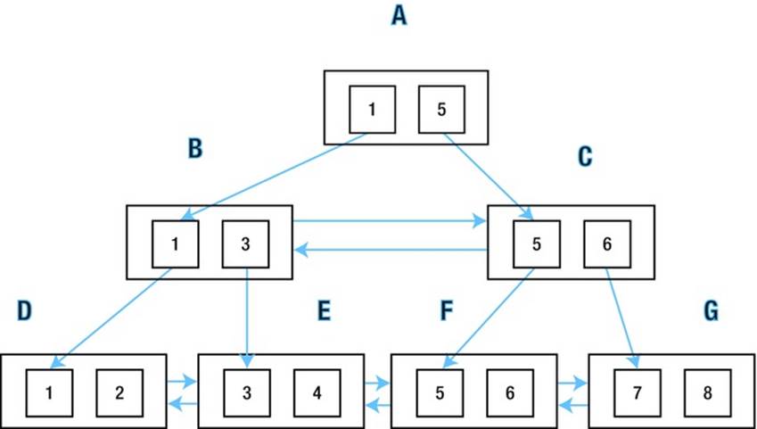
Figure 10-1. A simplified view of a B-tree index

Figure 10-1 depicts an index root block A, two branch blocks B and C, and four leaf blocks D, E, F, and G. I have drawn only two index entries per block. In real life there might be hundreds of entries. So if there were 200 entries per block there might be one root block, 200 branch blocks, 40,000 leaf blocks, and 8,000,000 index entries in those leaf blocks.

An INDEX FULL SCAN begins at the root of the index: block A in Figure 10-1. We use pointers in the blocks to descend the left side of the index structure until we have the block containing the smallest value of our leading indexed column, block D. We then follow the forward pointers along the leaf nodes visiting E, F, and G.

The index scan creates an intermediate result set containing rows with all the columns in the index and the ROWID. Of course if there are selection predicates in our WHERE clause (or predicates in the FROM list that can be treated as selection predicates) then we can filter out rows as we go. And equally clearly, we can discard any columns that we don’t need and create new columns based on expressions in our select list.

If the only columns we want from this table are in the index, we don’t need to do anything more. We are done. However, most of the time we will use the ROWID to access the associated table, table partition, or table subpartition using a TABLE ACCESS BY [LOCAL|GLOBAL] INDEX ROWID operation.

Be aware of the following:

· The layout of the blocks in the diagram is purely a logical sequence. The order on disk may be quite different.

· Because of this we must use single-block reads and follow the pointers. This can slow things down.

· The order of rows returned by an INDEX FULL SCAN is automatically sorted by the indexed columns, so this access method may avoid a sort. This can speed things up.

Listing 10-3 is an example of an INDEX FULL SCAN forced with the use of the INDEX hint:

Listing 10-3. INDEX FULL SCAN operation

CREATE INDEX t1_i1
ON t1 (c1, c2);

SELECT /*+ index(t1 (c1,c2)) */ * FROM t1;

---------------------------------------------
| Id | Operation | Name |
---------------------------------------------
| 0 | SELECT STATEMENT | |
| 1 | TABLE ACCESS BY INDEX ROWID| T1 |
| 2 | INDEX FULL SCAN | T1_I1 |
---------------------------------------------

Listing 10-3 creates a multi-column index on T1. The select statement includes a hint that specifies the use of the index.

Note Notice that the name of the index isn’t used in the hint. It is legal, and indeed encouraged, to specify the columns in the index you want to use, enclosed in parentheses, rather than the index name itself. This is to ensure that hints don’t break if somebody renames an index. All index hints displayed in the OUTLINE section of an execution plan use this approach.

Under certain circumstances the optimizer can make a huge improvement here and do something completely different under the guise of what is supposedly an INDEX FULL SCAN. Listing 10-4 shows an aggregate operation in use on an indexed column:

Listing 10-4. INDEX FULL SCAN with MIN/MAX optimization

SELECT /*+ index(t1 (c1,c2)) */
MAX (c1) FROM t1;

--------------------------------------------
| Id | Operation | Name |
--------------------------------------------
| 0 | SELECT STATEMENT | |
| 1 | SORT AGGREGATE | |
| 2 | INDEX FULL SCAN (MIN/MAX)| T1_I1 |
--------------------------------------------

What actually happens in Listing 10-4 is that we move down from the root block in our index using the trailing edge of the tree. In this case that would be A, C, and G. We can identify the maximum value of C1 straightaway without scanning the whole index. Don’t worry about the SORT AGGREGATE. As I explained in Chapter 3, the SORT AGGREGATE operation never sorts.

There are many restrictions and special cases that I researched for Oracle Database 10g in my blog in September 2009, seen here:

http://tonyhasler.wordpress.com/2009/09/08/index-full-scan-minmax/

I suspect this is a moving target and that much of what I said back then may not apply in later versions of Oracle Database, so if you are looking for this operation and can’t get it to work, you may just have to fiddle around a bit with your predicates.

There is also an INDEX FULL SCAN DESCENDING operation. This just starts off with the maximum value and works its way back through the index using the backward pointers. The difference is that the rows come back in descending order, which can avoid a sort, as Listing 10-5shows.

Listing 10-5. INDEX FULL SCAN DESCENDING

SELECT /*+ index_desc(t1 (c1,c2)) */
*
FROM t1
ORDER BY c1 DESC, c2 DESC;

---------------------------------------------
| Id | Operation | Name |
---------------------------------------------
| 0 | SELECT STATEMENT | |
| 1 | TABLE ACCESS BY INDEX ROWID| T1 |
| 2 | INDEX FULL SCAN DESCENDING| T1_I1 |
---------------------------------------------

Notice the absence of a sort operation despite the presence of the ORDER BY clause. Now, let us move on to the next access method in our list.

INDEX RANGE SCAN

The INDEX RANGE SCAN is very similar to the INDEX FULL SCAN. So similar, in fact, that the same hint is used to select it. The difference is that when a suitable predicate on one or more leading columns of the index is present in the query block we might be able to start our scan of leaf blocks somewhere in the middle and/or stop somewhere in the middle. In our diagram above, a predicate C1 BETWEEN 3 AND 5 would enable us to go from the root block A down to B, read E and F, and then stop. Listing 10-6 demonstrates:

Listing 10-6. INDEX RANGE SCAN

SELECT /*+ index(t1 (c1,c2)) */
*
FROM t1
WHERE c1 BETWEEN 3 AND 5;

---------------------------------------------
| Id | Operation | Name |
---------------------------------------------
| 0 | SELECT STATEMENT | |
| 1 | TABLE ACCESS BY INDEX ROWID| T1 |
| 2 | INDEX RANGE SCAN | T1_I1 |
---------------------------------------------

Performing an INDEX FULL SCAN when an INDEX RANGE SCAN is available never makes sense and the optimizer will never select it. I guess this is the reason that a separate hint for the INDEX RANGE SCAN hasn’t been documented.

There are some who would recommend the use of the alternative, undocumented INDEX_RS_ASC hint as it is more specific. Personally, I have no qualms whatsoever about using an undocumented hint, but I don’t see the point when a documented one exists!

The same comments I made about INDEX FULL SCANS apply to INDEX RANGE SCANS.

· We must use single-block reads and follow the pointers. This can slow things down.

· The order of rows returned by an INDEX RANGE SCAN is automatically sorted by the indexed columns, so this access method may avoid a sort. This can speed things up.

INDEX RANGE SCAN DESCENDING is the descending variant of INDEX RANGE SCAN and is shown in Listing 10-7.

Listing 10-7. INDEX RANGE SCAN DESCENDING

SELECT /*+ index_desc(t1 (c1,c2)) */
*
FROM t1
WHERE c1 BETWEEN 3 AND 5
ORDER BY c1 DESC;

----------------------------------------------
| Id | Operation | Name |
----------------------------------------------
| 0 | SELECT STATEMENT | |
| 1 | TABLE ACCESS BY INDEX ROWID | T1 |
| 2 | INDEX RANGE SCAN DESCENDING| T1_I1 |
----------------------------------------------

Listing 10-8 shows that the MIN/MAX optimization can be used with a range scan as with an INDEX FULL SCAN.

Listing 10-8. INDEX RANGE SCAN with MIN/MAX optimization

SELECT /*+ index(t1 (c1,c2)) */
MIN (c2)
FROM t1
WHERE c1 = 3
ORDER BY c1 DESC;

----------------------------------------------
| Id | Operation | Name |
----------------------------------------------
| 0 | SELECT STATEMENT | |
| 1 | SORT AGGREGATE | |
| 2 | FIRST ROW | |
| 3 | INDEX RANGE SCAN (MIN/MAX)| T1_I1 |
----------------------------------------------

Notice the sudden appearance of an extra operation—FIRST ROW. This sometimes pops up when the MIN/MAX optimization is used. I haven’t worked out what it means yet, and I suggest you just ignore it.

The INDEX RANGE SCAN requires there to be a suitable predicate on the leading column of the index. What happens when there are one or more predicates on non-leading columns but no predicate on the leading column? The INDEX SKIP SCAN is an option in this case.

INDEX SKIP SCAN

If the number of distinct values of the leading column is low, then a series of range scans, one for each value of the leading column, may be more efficient than an INDEX FULL SCAN. When the value of the leading column changes, the INDEX SKIP SCAN operation moves back up the B-tree and then descends again looking for the range associated with the new value of the leading column. Listing 10-9 demonstrates the operation.

Listing 10-9. INDEX SKIP SCAN

SELECT /*+ index_ss(t1 (c1,c2)) */
*
FROM t1
WHERE c2 = 3
ORDER BY c1, c2;

---------------------------------------------
| Id | Operation | Name |
---------------------------------------------
| 0 | SELECT STATEMENT | |
| 1 | TABLE ACCESS BY INDEX ROWID| T1 |
| 2 | INDEX SKIP SCAN | T1_I1 |
---------------------------------------------

Listing 10-10 shows the descending variant.

Listing 10-10. INDEX SKIP SCAN DESCENDING

SELECT /*+ index_ss_desc(t1 (c1,c2)) */
*
FROM t1
WHERE c2 = 3
ORDER BY c1 DESC, c2 DESC;

---------------------------------------------
| Id | Operation | Name |
---------------------------------------------
| 0 | SELECT STATEMENT | |
| 1 | TABLE ACCESS BY INDEX ROWID| T1 |
| 2 | INDEX SKIP SCAN DESCENDING| T1_I1 |
---------------------------------------------

Incidentally, in Oracle Database 10g it was not possible to request that an index be used AND say that an INDEX SKIP SCAN NOT be used. This is no longer true. Just use an INDEX hint and you will get an INDEX FULL SCAN.

INDEX UNIQUE SCAN

The INDEX UNIQUE SCAN is used when accessing at most one row from a unique index. This is a separate operation because it is implemented in a more efficient way than reading a row from a non-unique index that happens to only have one row. Listing 10-11 creates a unique index and then shows the operation.

Listing 10-11. INDEX UNIQUE SCAN

CREATE UNIQUE INDEX t1_i2
ON t1 (c2);

SELECT /*+ index(t1 (c2)) */
*
FROM t1
WHERE c2 = 1;

---------------------------------------------
| Id | Operation | Name |
---------------------------------------------
| 0 | SELECT STATEMENT | |
| 1 | TABLE ACCESS BY INDEX ROWID| T1 |
| 2 | INDEX UNIQUE SCAN | T1_I2 |
---------------------------------------------

Notice that there is no “descending” variant of this plan because we are retrieving only one row.

INDEX FAST FULL SCAN

The next indexed access method is the INDEX FAST FULL SCAN. Well, we like that word fast, don’t we? The obvious question is: If we have a full scan that is fast, why do we need the slow one? The truth is that the INDEX FAST FULL SCAN has one big restriction and is not always faster than a regular INDEX FULL SCAN.

An INDEX FAST FULL SCAN reads the whole index with multi-block reads. Forget about all those pesky pointers. Just suck the whole index in!

Of course, multi-block reads are always a faster way to read a lot of data than single-block reads. However:

· We are reading all the data in the index—not just the leaf blocks we need.

· The data is provided in physical order, not logical order.

As to the first point, it doesn’t matter too much. Nearly all the blocks in an index are leaf blocks anyway, so we are only throwing away a small portion. As to the second point, we may not be interested in the order. Even if we are interested in the order, combining an INDEX FAST FULL SCAN with an explicit sort may be cheaper than alternative access methods.

The really disappointing thing about the INDEX FAST FULL SCAN is that unlike all the other index access methods discussed so far we can’t use the ROWIDs to access the table. As to why the developers have imposed this restriction, I have no idea.

If you are reading this because you have just received a call due to a performance problem and suspect that an INDEX FAST FULL SCAN with subsequent table access would help you, skip ahead to Chapter 19, where I document a workaround.

Listing 10-12 shows the operation.

Listing 10-12. INDEX FAST FULL SCAN

SELECT /*+ index_ffs(t1 (c1, c2)) */
c1, c2
FROM t1
WHERE c2 = 1;

--------------------------------------
| Id | Operation | Name |
--------------------------------------
| 0 | SELECT STATEMENT | |
| 1 | INDEX FAST FULL SCAN| T1_I1 |
--------------------------------------

This example demonstrates that we don’t necessarily need all the rows in the index to use an INDEX FAST FULL SCAN; our WHERE clause is free to dispose of some of them. Of course, if you want to use an index but do not want to use a fast full scan, use the INDEX orINDEX_DESC hints.

INDEX SAMPLE FAST FULL SCAN

The final index access method that uses just one B-tree index is probably most used by the DBMS_STATS package when gathering index statistics. It is only used when taking samples in combination with a fast full scan. Listing 10-13 demonstrates.

Listing 10-13. INDEX SAMPLE FAST FULL SCAN

SELECT /*+ index_ffs(t1 (c1, c2)) */
c1, c2
FROM t1 SAMPLE (5);

---------------------------------------------
| Id | Operation | Name |
---------------------------------------------
| 0 | SELECT STATEMENT | |
| 1 | INDEX SAMPLE FAST FULL SCAN| T1_I1 |
---------------------------------------------

All the access methods discussed so far involve only a single B-tree index. There are two access methods available in all editions of Oracle database that allow B-tree indexes to be combined. Let us look at the first of these now.

INDEX JOIN

Listing 10-14 shows an example of an INDEX JOIN using tables from the HR example schema.

Listing 10-14. Index join example

SELECT
e.first_name
FROM hr.employees e
WHERE e.manager_id >=100 AND e.last_name LIKE '%ran%';

---------------------------------------------------
| Id | Operation | Name |
---------------------------------------------------
| 0 | SELECT STATEMENT | |
|* 1 | VIEW | index$_join$_001 |
|* 2 | HASH JOIN | |
|* 3 | INDEX RANGE SCAN | EMP_MANAGER_IX |
|* 4 | INDEX FAST FULL SCAN| EMP_NAME_IX |
---------------------------------------------------

Listing 10-14 joins two indexes on the EMPLOYEES tables as if they were themselves tables. The joined column is the ROWID from the table. What has effectively happened is that Listing 10-14 has been transformed into Listing 10-15.

Listing 10-15. Manually transformed index join

WITH q1
AS (SELECT /*+ no_merge */ first_name, ROWID r1
FROM hr.employees
WHERE last_name LIKE '%ran%')
,q2
AS (SELECT /*+ no_merge */ ROWID r2
FROM hr.employees
WHERE manager_id >=100)
SELECT first_name
FROM q1, q2
WHERE r1 = r2;

Subquery Q1 in Listing 10-15 can be satisfied by a range scan on the EMP_NAME_IX index with no need to access the table itself, as the only columns we are selecting come from the index. Subquery Q2 can similarly restrict its access to the EMP_MANAGER_IX index. The main query then joins the results of the two subqueries using the ROWIDs from the two indexes.

Be aware that an index join is only possible if the only columns required from the table whose indexes are being joined are those present in the indexes. However, it is possible to combine index joins with regular table joins under certain circumstances, as demonstrated in Listing 10-16.

Listing 10-16. Complex INDEX JOIN example

SELECT /*+ leading(e) index_join(e) */
e.first_name, m.last_name
FROM hr.employees e, hr.employees m
WHERE m.last_name = 'Mourgos'
AND e.manager_id = m.employee_id
AND e.last_name = 'Grant'
AND e.department_id = 50;
----------------------------------------------------------
| Id | Operation | Name |
----------------------------------------------------------
| 0 | SELECT STATEMENT | |
| 1 | NESTED LOOPS | |
| 2 | NESTED LOOPS | |
|* 3 | VIEW | index$_join$_001 |
|* 4 | HASH JOIN | |
|* 5 | HASH JOIN | |
|* 6 | INDEX RANGE SCAN | EMP_DEPARTMENT_IX |
|* 7 | INDEX RANGE SCAN | EMP_NAME_IX |
| 8 | INDEX FAST FULL SCAN | EMP_MANAGER_IX |
|* 9 | INDEX UNIQUE SCAN | EMP_EMP_ID_PK |
|* 10 | TABLE ACCESS BY INDEX ROWID| EMPLOYEES |
----------------------------------------------------------

Since there are only two employees with a surname of Grant and only one of these with Mourgos as a manager, an index join is not suitable on performance grounds for this particular query, but we can use hints for demonstration purposes.

Notice that the reference to M.LAST_NAME doesn't prohibit the index join as it doesn’t come from the copy of the EMPLOYEES table with table alias E.

· Index joins require that only columns in the indexes being joined are referenced. You can’t even reference the ROWID!

· Index joins are only possible on the first table in a set of joined tables (hence the LEADING hint above).

· Index joins can be forced (when legal) with the INDEX_JOIN hint as in Listing 10-16 above.

If you do see index joins happening a lot you might want to consider creating a multi-column index, as this will be slightly more efficient than the index join, but in my experience index joins aren’t usually the source of serious performance issues.

You might think that an index join might sometimes be suitable even when you do want to reference rows in the main table. Well, there is a way to do this.

AND_EQUAL

Listing 10-17 shows the AND_EQUAL access method, but the optimizer will no longer use it unless hinted and that hint is deprecated.

Listing 10-17. Depreccated AND_EQUAL access method

SELECT /*+ and_equal(e (manager_id) (job_id)) */
employee_id
,first_name
,last_name
,email
FROM hr.employees e
WHERE e.manager_id = 124 AND e.job_id = 'SH_CLERK';

------------------------------------------------------
| Id | Operation | Name |
------------------------------------------------------
| 0 | SELECT STATEMENT | |
|* 1 | TABLE ACCESS BY INDEX ROWID| EMPLOYEES |
| 2 | AND-EQUAL | |
|* 3 | INDEX RANGE SCAN | EMP_MANAGER_IX |
|* 4 | INDEX RANGE SCAN | EMP_JOB_IX |
------------------------------------------------------

Listing 10-17 shows the two sets of ROWIDs being merged as before (but perhaps using a different mechanism), but then we use the ROWIDs to access the table and pick up the additional columns.

· This is a deprecated feature.

· There are numerous restrictions, one of which is that the indexes must be single-column, non-unique indexes.

· It requires the AND_EQUAL hint. The optimizer will never generate this plan unless hinted.

· This mechanism will rarely provide a performance improvement, but if it does then a multi-column index is usually warranted.

· There are alternative approaches for both standard edition users and enterprise edition users. We will discuss an option for standard edition users in Chapter 19. The next section on bitmap indexes shows several ways to combine indexes for enterprise edition users.

Bitmap Index Access

The physical structure of a bitmap index is actually very similar to that of a B-tree index, with the root and branch block structures being identical.

The difference comes at the leaf block. Let us suppose that we have a B-tree index on column C1 on T1 and that there are 100 rows in T1 that have a value of 'X' for C1. The B-tree index would contain 100 index entries, each with a ROWID for a particular matching row in the table.

The bitmap index would instead have a bitmap for value 'X' that had one bit for every row in the table or partition; for the 100 rows in the table with value 'X' for C1 the bit would be set, but it would be clear for the remaining rows.

These bitmaps in the leaf blocks are compressed to remove long stretches of clear bits so the more clustered the data in the table is, the smaller the index is. This compression generally means that even if there is an average of only two rows for each value, the bitmap index will be smaller than its B-tree counterpart.

You should always remember that bitmaps are representations of collections of restricted ROWIDs. It is, therefore, not possible to

· create a global bitmap index;

· convert ROWIDs from a global index into a bitmap; or

· convert variables or expressions of type ROWID or UROWID to bitmaps.

The operations to access a bitmap index are, unsurprisingly, similar to those for a B-tree index (see Table 10-3).

Table 10-3. Bitmap-indexed access operations

Looking at Table 10-3 you will notice the following

· There are no descending or skip scan variants.

· There are no MIN/MAX optimizations available.

· There is no UNIQUE option—hardly surprising as the silly idea of a unique bitmap index isn’t even supported.

The BITMAP INDEX SINGLE VALUE operation is used when an equality predicate is supplied for the column or columns in the index and implies the processing of a single bitmap.

The BITMAP CONSTRUCTION and BITMAP COMPACTION are provided for completeness. If you run EXPLAIN PLAN on a CREATE BITMAP INDEX or ALTER INDEX...REBUILD command you will see these operations appear. They are DDL specific.

We can do a whole lot more with bitmaps other than just accessing them in indexes. Table 10-4 shows the full set of operations.

Table 10-4. Bitmap manipulation operations

The operation BITMAP CONVERSION FROM ROWIDS is used to convert restricted ROWIDs from a B-tree index into a bitmap, and the operation BITMAP CONVERSION TO ROWIDS is used to convert bitmaps to restricted ROWIDs.

The BITMAP AND, BITMAP OR, and BITMAP MINUS operations perform Boolean algebra operations in the expected way; complex trees of bitmap operations can be formed. The BITMAP MERGE operation is similar to BITMAP OR but is used in some contexts where the ROWID sets are known to be disjointed.

Usually, after all this manipulation of bitmaps, the final result is passed to the BITMAP CONVERSION TO ROWIDS operation. However, sometimes all we want is a count of the number of rows. This can be done by the BITMAP CONVERSION COUNT operation.

The BITMAP KEY ITERATION operation is used in star transformations, which we will discuss in Chapter 13.

It is not unusual to see a lot of bitmap operations in one query, as in Listing 10-18.

Listing 10-18. Bitmap operations

CREATE INDEX t1_i3
ON t1 (c5);

CREATE BITMAP INDEX t1_bix1
ON t1 (c3);

SELECT /*+ index_combine(t)no_expand */
*
FROM t1 t
WHERE (c1 > 0 AND c5 = 1 AND c3 > 0) OR c4 > 0;

-----------------------------------------------------
| Id | Operation | Name |
-----------------------------------------------------
| 0 | SELECT STATEMENT | |
| 1 | TABLE ACCESS BY INDEX ROWID | T1 |
| 2 | BITMAP CONVERSION TO ROWIDS | |
| 3 | BITMAP OR | |
| 4 | BITMAP MERGE | |
| 5 | BITMAP INDEX RANGE SCAN | T1_BIX2 |
| 6 | BITMAP AND | |
| 7 | BITMAP CONVERSION FROM ROWIDS| |
| 8 | INDEX RANGE SCAN | T1_I3 |
| 9 | BITMAP MERGE | |
| 10 | BITMAP INDEX RANGE SCAN | T1_BIX1 |
| 11 | BITMAP CONVERSION FROM ROWIDS| |
| 12 | SORT ORDER BY | |
| 13 | INDEX RANGE SCAN | T1_I1 |
-----------------------------------------------------

Listing 10-18 begins by creating two more indexes. The execution plan for the query looks a bit scary, but the first thing to understand when reading execution plans like this is that you should not panic. You can follow them easily enough if you take it step by step.

Let us start at operation 5, which is the first operation without a child. This performs a BITMAP INDEX RANGE SCAN on T1_BIX2, which is based on column C4. This range scan will potentially process multiple bitmaps associated with different values of C4, and these are merged by operation 4. This merged bitmap represents the first operand of the BITMAP OR on line 3. We then move on to look at the second operand of the BITMAP OR, which is defined by the operation on line 6 as well as its children.

We now look at operation 8, which is the second operation with no child. This is an INDEX RANGE SCAN on T1_I3, which is a B-tree index based on C5. In this case we have an equality predicate, C5 = 1, and that means all the rows returned have the same index key. A little known fact is that entries from a non-unique index that have the same key value are sorted by ROWID. This means that all the rows returned by the INDEX RANGE SCAN will be in ROWID order and can be directly converted to a bitmap by operation 7. This BITMAP MERGE forms the first operand of the BITMAP AND operation on line 6.

We move on to line 10, an INDEX RANGE SCAN on T1_BIX1, a bitmap index based on C3. Once again, multiple values of C3 are possible and so the various bitmaps need to be merged by line 9, finalizing the second operand of operation 6, the BITMAP AND.

But there is a third operand of operation 6. We begin the evaluation of this third operand by looking at line 13, an INDEX RANGE SCAN on T1_I1, a B-tree index on C1 and C2. Because the range scan may cover multiple key values, the index entries may not be returned in ROWID order; we need to sort the ROWIDs on line 12 before converting them into a bitmap on line 11.

We now have the three operands to the BITMAP AND operation on line 6 and the two operands to the BITMAP OR operation on line 3. After all bitmap manipulation, the final bitmap is converted to a set of ROWIDs on line 2, and these are finally used to access the table on line 1.

Listing 10-19 changes Listing 10-18 slightly to return the count of rows rather than the contents; we can see that the conversion of the bitmap to ROWIDs can be eliminated.

Listing 10-19. BITMAP CONVERSION COUNT example

SELECT /*+ index_combine(t) */
COUNT (*)
FROM t1 t
WHERE (c1 > 0 AND c5 = 1 AND c3 > 0) OR c4 > 0;

-----------------------------------------------------
| Id | Operation | Name |
-----------------------------------------------------
| 0 | SELECT STATEMENT | |
| 1 | SORT AGGREGATE | |
| 2 | BITMAP CONVERSION COUNT | |
| 3 | BITMAP OR | |
| 4 | BITMAP MERGE | |
| 5 | BITMAP INDEX RANGE SCAN | T1_BIX2 |
| 6 | BITMAP AND | |
| 7 | BITMAP MERGE | |
| 8 | BITMAP INDEX RANGE SCAN | T1_BIX1 |
| 9 | BITMAP CONVERSION FROM ROWIDS| |
| 10 | INDEX RANGE SCAN | T1_I3 |
| 11 | BITMAP CONVERSION FROM ROWIDS| |
| 12 | SORT ORDER BY | |
| 13 | INDEX RANGE SCAN | T1_I1 |
-----------------------------------------------------

The main difference between this plan and the last one is the presence of the BITMAP CONVERSION COUNT operation on line 2 and the absence of any BITMAP CONVERSION TO ROWIDS operation.

One major restriction of bitmap operations, which we will investigate in detail when we discuss the star transformation in Chapter 13, is that this mechanism cannot deal with “in lists” with subqueries such as is unsuccessfully attempted in Listing 10-20.

Listing 10-20. INDEX COMBINE attempt with INLIST

SELECT /*+ index_combine(e) */
/* THIS HINT INNEFFECTIVE IN THIS QUERY */
employee_id
,first_name
,last_name
,email
FROM hr.employees e
WHERE manager_id IN (SELECT employee_id
FROM hr.employees
WHERE salary > 14000)
OR job_id = 'SH_CLERK';

------------------------------------------------------
| Id | Operation | Name |
------------------------------------------------------
| 0 | SELECT STATEMENT | |
| 1 | FILTER | |
| 2 | TABLE ACCESS BY INDEX ROWID| EMPLOYEES |
| 3 | INDEX FULL SCAN | EMP_EMP_ID_PK |
| 4 | TABLE ACCESS BY INDEX ROWID| EMPLOYEES |
| 5 | INDEX UNIQUE SCAN | EMP_EMP_ID_PK |
------------------------------------------------------

Full Table Scans

We now come to the pariah of operations in an execution plan: the much maligned full table scan (see Table 10-5).

Table 10-5. Full table scan operations

Although we all refer to the operation as a full table scan, the actual name of the operation in an execution plan display is TABLE ACCESS FULL. Both terms are slightly misleading because in the case of a partitioned table, the “table” being scanned is actually an individual partition or subpartition. Perhaps to avoid an over-specific term it might have been called “segment full scan,” but that wouldn’t be specific enough; we aren’t talking about indexes here, after all. To keep it simple I will assume that we are looking at non-partitioned tables for the remainder of this section; the mechanics don’t change. I’ll also use the abbreviation FTS for brevity.

The FTS operation sounds simple enough: we read all the blocks in the table from beginning to end.

However, it is actually a lot more complicated than that. We need to

· access the segment header to read the extent map and identify the high water mark (HWM);

· read all the data in all the extents up to the HWM; and

· re-read the segment header to confirm that there are no more rows.

Even if we are talking only about serial, as opposed to parallel, operations, that still isn’t the full story. Once all the data has been returned to the client an extra FETCH operation may be required to reconfirm that there is no more data. That will result in a third read of the segment header.

These extra reads of the segment header aren’t usually a major factor when we are looking at a large, or even medium-sized, table, but for a tiny table of, say, one block these extra reads might be an issue. If the tiny table is frequently accessed you may need to create an index or just convert the table to an index-organized table.

Some people will tell you that the key to tuning badly performing SQL is to search out FTSs and eliminate them by adding indexes. This is a dangerous half-truth. It is certainly the case that a missing index can cause performance problems and that those performance problems might be recognized by the presence of a TABLE FULL SCAN operation in an execution plan. However, FTSs are very often the most efficient way to access a table, as I explained when I introduced the concept of the index clustering factor in Chapter 9. If you have forgotten, take a look back atFigure 9-1.

Listing 10-21 shows the basic FTS operation in action.

Listing 10-21. FULL TABLE SCAN

SELECT /*+ full(t1) */
* FROM t1;

----------------------------------
| Id | Operation | Name |
----------------------------------
| 0 | SELECT STATEMENT | |
| 1 | TABLE ACCESS FULL| T1 |
----------------------------------

Listing 10-22 shows the second operation listed at the top of this section. As with INDEX FAST FULL SCAN, the use of a sample changes the operation.

Listing 10-22. TABLE ACCESS SAMPLE

SELECT /*+ full(t1) */
*
FROM t1 SAMPLE (5);

------------------------------------
| Id | Operation | Name |
------------------------------------
| 0 | SELECT STATEMENT | |
| 1 | TABLE ACCESS SAMPLE| T1 |
------------------------------------

Listing 10-22 requests a 5 percent sample from the table. The final FTS variant is demonstrated in Listing 10-23, which shows a query with parallel sampling.

Listing 10-23. TABLE ACCESS SAMPLE in parallel

SELECT /*+ full(t1) parallel */
*
FROM t1 SAMPLE (5);

----------------------------------------------------------
| Id | Operation | Name |
----------------------------------------------------------
| 0 | SELECT STATEMENT | |
| 1 | PX COORDINATOR | |
| 2 | PX SEND QC (RANDOM) | :TQ10000 |
| 3 | PX BLOCK ITERATOR | |
| 4 | TABLE ACCESS SAMPLE BY ROWID RANGE| T1 |
----------------------------------------------------------

TABLE and XMLTABLE

The list of functions in the SQL Language Reference manual includes XMLTABLE. For reasons that will shortly become clear, I will inaccurately refer to XMLTABLE as an “operator.” A sibling to XMLTABLE is TABLE, but that “operator” is curiously documented in a completely different part of the manual than XMLTABLE.

The XMLTABLE “operator” has an Xquery “operand,” and the result of the “operation” is a row source that can appear in a FROM clause just like a regular table or view.

I am not an XML guru, but Listing 10-24 is a quick example of the use of XMLTABLE.

Listing 10-24. XMLTABLE example

CREATE TABLE xml_test (c1 XMLTYPE);

SELECT x.*
FROM xml_test t
,XMLTABLE (
'//a'
PASSING t.c1
COLUMNS "a" CHAR (10) PATH '@path1'
,"b" CHAR (50) PATH '@path2'
) x;

---------------------------------------
| Id | Operation | Name |
---------------------------------------
| 0 | SELECT STATEMENT | |
| 1 | NESTED LOOPS | |
| 2 | TABLE ACCESS FULL| XML_TEST |
| 3 | XPATH EVALUATION| |
---------------------------------------

The TABLE “operator” has an “operand” that is a nested table. The nested table operand has one of three formats:

· A data dictionary or casted PL/SQL nested table object

· A function that returns a nested table object. Such functions are typically pipelined functions

· A CAST...MULTISET expression

The second of these three forms is the most common, and the pipelined functions are often referred to as “table functions.” This common use of the term “table function” makes it easier to refer to the keywords TABLE and XMLTABLE as “operators” rather than functions.

Nested tables in the data dictionary aren’t a very good idea. The tables themselves aren’t stored inline and so you might as well have a child table with a referential integrity constraint linking it to the parent. This way you would at least have the option of accessing the child data without visiting the parent.

Note We will see in Chapter 13 that these days the CBO can perform the table elimination transformation so that any unnecessary reference to the parent table is eliminated.

However, if you have inherited some nasty nested tables from your predecessor, Listing 10-25 shows how you query them.

Listing 10-25. Querying a nested table

CREATE TYPE order_item AS OBJECT
(
product_name VARCHAR2 (50)
,quantity INTEGER
,price NUMBER (8, 2)
);
/

CREATE TYPE order_item_table AS TABLE OF order_item;
/

CREATE TABLE orders
(
order_id NUMBER PRIMARY KEY
,customer_id INTEGER
,order_items order_item_table
)
NESTED TABLE order_items
STORE AS order_items_nt;

SELECT o.order_id
,o.customer_id
,oi.product_name
,oi.quantity
,oi.price
FROM orders o, TABLE (o.order_items) oi;

----------------------------------------------------------------
| Id | Operation | Name |
----------------------------------------------------------------
| 0 | SELECT STATEMENT | |
| 1 | NESTED LOOPS | |
| 2 | NESTED LOOPS | |
| 3 | TABLE ACCESS FULL | ORDERS |
| 4 | INDEX RANGE SCAN | SYS_FK0000127743N00003$ |
| 5 | TABLE ACCESS BY INDEX ROWID| ORDER_ITEMS_NT |
----------------------------------------------------------------

As you can see, there is a nested loop from our newly created parent table ORDERS to our nested table ORDER_ITEMS_NT via an automatically created index on a hidden column. Other join orders and methods are possible.

Note Information about all columns, including column statistics, in nested tables can be seen in the view ALL_NESTED_TABLE_COLS. This view also shows the hidden NESTED_TABLE_ID column on which the index is built.

A pipelined table function is a much better use of the table operator. Listing 10-26 shows a common example.

Listing 10-26. DBMS_XPLAN.display example

SELECT * FROM TABLE (DBMS_XPLAN.display);

-----------------------------------------------------
| Id | Operation | Name |
-----------------------------------------------------
| 0 | SELECT STATEMENT | |
| 1 | COLLECTION ITERATOR PICKLER FETCH| DISPLAY |
-----------------------------------------------------

You can see the operation COLLECTION ITERATOR PICKLER FETCH to signify a call to the pipelined function to retrieve rows. In fact, these rows are batched so you don’t get a context switch between the calling SQL statement and the pipelined function for every row retrieved.

The third and final way to use the table operator is with a subquery. Listing 10-27 shows what may be somewhat unfamiliar syntax, and it requires the use of user-defined types to get it working.

Listing 10-27. CAST MULTISET example

SELECT *
FROM TABLE (CAST (MULTISET (SELECT 'CAMERA' product, 1 quantity, 1 price
FROM DUAL
CONNECT BY LEVEL <= 3) AS order_item_table)) oi;

---------------------------------------------------
| Id | Operation | Name |
---------------------------------------------------
| 0 | SELECT STATEMENT | |
| 1 | COLLECTION ITERATOR SUBQUERY FETCH| |
| 2 | COUNT | |
| 3 | CONNECT BY WITHOUT FILTERING | |
| 4 | FAST DUAL | |
---------------------------------------------------

Here I have queried DUAL to generate a collection of three rows and then cast the result into a nested table using the ORDER_ITEM_TYPE that I created in Listing 10-25. The table operator then allows me to treat this nested table as a row source. The query results are the same as that of the original SELECT from DUAL.

The execution plan in Listing 10-27 shows the subquery on lines 2, 3, and 4, while the COLLECTION ITERATOR SUBQUERY FETCH operation on line 1 has been generated by the TABLE operator.

This all seems very complicated and unnecessary. Why go to all the trouble of creating a nested table from a bunch of rows only to expand them back into rows? However, the use of this technique in combination with the left lateral joins that I touched on earlier can be very useful on some occasions, as we will see in Chapter 17.

Cluster Access

I need to mention clusters in this chapter for the sake of completeness (see Table 10-6).

Table 10-6. Cluster access operations

Let me go through this example. Listing 10-28 is the final in this chapter.

Listing 10-28. Cluster access methods

CREATE CLUSTER cluster_hash
(
ck INTEGER
)
HASHKEYS 3
HASH IS ck;

CREATE TABLE tch1
(
ck INTEGER
,c1 INTEGER
)
CLUSTER cluster_hash ( ck );

CREATE CLUSTER cluster_btree
(
ck INTEGER,
c1 INTEGER
);

CREATE INDEX cluster_btree_ix
ON CLUSTER cluster_btree;

CREATE TABLE tc2
(
ck INTEGER
,c1 INTEGER
)
CLUSTER cluster_btree ( ck, c1 );

CREATE TABLE tc3
(
ck INTEGER
,c1 INTEGER
)
CLUSTER cluster_btree ( ck, c1 );

SELECT /*+ hash(tch1) index(tc2) cluster(tc3)*/
*
FROM tch1, tc2, tc3
WHERE tch1.ck = 1
AND tch1.ck = tc2.ck
AND tch1.c1 = tc2.c1
AND tc2.ck = tc3.ck
AND tc2.c1 = tc3.c1;

---------------------------------------------------
| Id | Operation | Name |
---------------------------------------------------
| 0 | SELECT STATEMENT | |
| 1 | NESTED LOOPS | |
| 2 | NESTED LOOPS | |
| 3 | TABLE ACCESS HASH | TCH1 |
| 4 | TABLE ACCESS CLUSTER| TC2 |
| 5 | INDEX UNIQUE SCAN | CLUSTER_BTREE_IX |
| 6 | TABLE ACCESS CLUSTER | TC3 |
---------------------------------------------------

Listing 10-28 begins by creating a hash cluster, a B-tree cluster, and three associated tables. Table TCH1 is created in the single table hash cluster and tables TC2 and TC3 are created in the B-tree cluster.

The execution plan for the query in Listing 10-28 begins by accessing table TCH1. Because we included the predicate TCH1.CK = 1 in our query and CK is our hash cluster key, we are able to go directly to the block or blocks that contain the matching rows from TCH1 without the use of an index. For each of the matching rows in TCH1 we use the value of CK and C1 to access our cluster index on CLUSTER_BTREE. Cluster indexes are special in that they only have one entry per key value, hence why we get an INDEX UNIQUE SCAN operation on line 5 even though there may be many rows in TC2 that match the particular values of CK and C1 extracted from TCH1.

Because columns CK and C1 were both defined in CLUSTER_BTREE and were also specified as join conditions for TC2 and TC3, we know that the rows we want in TC3 are collocated with those of TC2. In fact, the single index entry lookup on line 5 helps us find all the rows we need in both TC2 and TC3 that match our row from TCH1.

All this looks pretty cool. In fact, clusters are used extensively in the data dictionary. However, I personally have never worked on any production Oracle database that has used any kind of cluster outside of the data dictionary.

So why are they so unpopular? Well, in the vast majority of cases the main overhead of accessing data through an index is in accessing the data in the table, not in doing the index lookup. This is because the index structure itself is likely to be cached and the table data may well not be. This tends to limit the benefit of hash clusters. Hash clusters are also a little difficult to manage because you have to know roughly how many rows will match each particular hash key. On the one hand, if you get this value too small then the hash chains become long. On the other hand, if you make the value too large then your cluster is unnecessarily large and you end up with more logical and/or physical I/O than you need. Whether you set the HASHKEYS parameter too large or too small, the performance benefit you thought you might get would rapidly disappear.

But what about regular B-tree clusters? You don’t have to worry about setting HASHKEYS, and you still get the main performance benefit of clusters, don’t you?

Imagine you have a table called ORDERS with a primary key, ORDER_ID, and an ORDER_ITEMS table with a referential integrity constraint linking it to the parent table. Wouldn’t it be nice to be able to make one single-block read and get one row from the ORDERS table and its corresponding rows from the ORDER_ITEMS table? Surely that is better than making two I/Os to retrieve the data from the two tables separately, isn’t it?

Well, yes. However, queries that retrieve data for just one order are going to complete quite quickly anyway, and you may not notice the performance improvement. On the other hand, if you are running a report that looks at large numbers of orders and their associated line items you are going to read lots of blocks anyway, so how the data is split between these blocks is of little consequence.

You may have a system with hundreds or thousands of interactive users, so the ORDERS and ORDER_ITEMS tables may be huge and unable to be cached in the SGA, so you really want to halve these I/Os to improve capacity.

Fine. Unfortunately, there is one big problem with this scenario: you can’t partition clustered tables. That is a big “gotcha.” Partitioning provides significant administrative and performance benefits for large tables, and few people are prepared to give them all up just to enjoy the benefits of clusters.

But if partitioning is out of the picture for you, perhaps because of licensing issues, and you frequently perform joins between tables as I have described, then clustering may seem like a good option.

Even in these rare circumstances, most people end up denormalizing their data or finding some other workaround rather than using something like a cluster that, rightly or wrongly, is viewed as a big unknown. I won’t be mentioning clusters again in this book.

Summary

I am afraid that even this lengthy discussion of access methods is incomplete. We haven’t discussed access to LOB objects, use of REF data types, or the use of domain indexes. But even so, this chapter has covered all the access methods that you are likely to encounter in the vast majority of SQL statements in commercial applications.

Having covered the various ways to access a single row source within a query it is now time to turn our attention to the topic of joining these row sources together. On to Chapter 11.