Expert Oracle SQL: Optimization, Deployment, and Statistics (2014)
PART 4. Optimization
CHAPTER 17. Optimizing Sorts
I speculate that in the 1980s and 1990s the biggest source of SQL performance problems was probably poor join order. If you made the wrong choice of table to start your joins you would likely end up in a world of pain. These days we have a reasonably mature CBO and a sophisticated runtime engine that between them support right-deep join trees, star transformations, and a wealth of other fancy features. On the one hand, these improvements mean that join order is much less of a problem for those of us working with an Oracle database than it was. On the other hand, I seem to spend a lot of time these days sorting out sorts. All too often a SQL statement will apparently hang and gobble up all the temporary table space, bringing the entire database to a screeching halt. This chapter is dedicated entirely to the important topic of optimizing sorts and for the most part focuses on writing or rewriting SQL efficiently.
Sort optimization is almost entirely about one thing: stopping the sort from spilling to disk. And if you can’t stop the sort from spilling to disk then you need to minimize the amount of disk activity that occurs. There are really only four ways to achieve this goal:
· Don’t sort at all. Or sort less often. The most efficient sort is the one you don’t do.
· Sort fewer columns. Fewer columns means less demand for memory.
· Sort fewer rows. Fewer rows means less demand on memory and fewer comparisons as well.
· Grab more memory for your sorts.
These concepts are easy enough to grasp, but achieving them is often quite tough. Before we get started on optimization let us review the basic mechanism that Oracle uses for sorting large amounts of data.
The Mechanics of Sorting
When we think of sorting most of us instinctively think about the ORDER BY clause. But sorting occurs in a number of other places as well. Sort merge joins, aggregate functions, analytic functions, set operations, model clauses, hierarchical queries, index builds and rebuilds and anything else that I have forgotten all involve sorts. All these sorting requirements are satisfied using variations of the same basic sort mechanism.
If you can sort all your rows in memory the sort is referred to as optimal. But what happens if you try and sort your data and it won’t fit into memory without blowing the limit that the runtime engine has set? At some point your sort will spill to disk. In this section I want to talk about what happens when a sort cannot be fully achieved in memory. But first let me talk briefly about how limits on memory allocation are set.
Memory Limits for Sorts
Sorts are initially performed in an in-memory workarea. The upper limit on the size of this workarea is mainly controlled, indirectly, by the four initialization parameters: MEMORY_TARGET, PGA_AGGREGATE_TARGET, WORKAREA_SIZE_POLICY, and SORT_AREA_SIZE. The last two of these four parameters can be set at the session level.
If WORKAREA_SIZE_POLICY is set to AUTO then PGA_AGGREGATE_TARGET (or MEMORY_TARGET, if set) indirectly tries to regulate Program Global Area (PGA) memory allocations including workareas: as more memory is allocated by sessions in the instance the less memory will be allocated for new workareas. If you set WORKAREA_SIZE_POLICY to MANUAL (and you can do this at the session level) you have full control over the limits on workarea allocation. Generally it is a good idea to leave WORKAREA_SIZE_POLICY set to AUTO. However, you should set WORKAREA_SIZE_POLICY to MANUAL when you have a critical batch process that you know will be running at a quiet time of the day (or night) and that will need to allocate a substantial proportion of the available memory.
The algorithms for calculating the amount of memory for a workarea change from release to release, but the following statements apply to 11gR2 (at least):
· The maximum amount of memory that can be allocated to a workarea when the value of WORKAREA_SIZE_POLICY is set to the default value of AUTO is 1GB no matter how big PGA_AGGREGATE_TARGET is.
· The maximum amount of memory that can be allocated to a workarea when you set WOKAREA_SIZE_POLICY to MANUAL is just under 2GB.
· You can allocate more memory to a sort by using parallel query, as each parallel query slave gets its own workarea. However, once you have more than six parallel query slaves the amount of memory allocated to each parallel query slave is reduced to prevent the amount of memory allocated to a specific sort from getting any bigger. This implies that no matter what you do you can’t allocate more than 12GB to any one sort.
Of course, these high numbers can’t always be achieved. For one thing, a SQL statement may have more than one workarea active at once, and there are various undocumented limits that change from release to release that limit the total amount of memory that can be allocated to all workareas in a process at one time. Let me now discuss what happens when you can’t get enough memory for your sort.
Disk-based Sorts
As rows are added to the in-memory workarea they are maintained in sorted order. When the in-memory workarea is full some of the sorted rows are written to the designated temporary tablespace. This disk-based area is known as a sort run. Once the sort run has been written to disk, memory is freed up for more rows. This process can be repeated many times until all the rows have been processed. Figure 17-1 illustrates how this works:
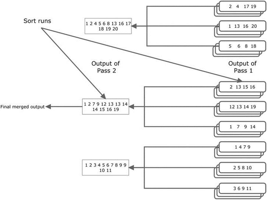
Figure 17-1. A two-pass sort
The nine boxes on the right of Figure 17-1 represent nine sort runs. The numbers in the boxes represent sorted rows, although in reality there would normally be many more than four rows in a sort run. Once all the sort runs have been created the first few blocks of each sort run are read back into memory, merged, and output. As the merged rows are output memory is freed up and more data can be read in from disk. This flavor of sort is referred to as a one-pass sort as each row is written to disk and read back just once.
However, what happens when there aren’t nine sort runs generated by our first pass but 9,000? At that point you may not be able to fit even one block from all 9,000 sort runs into your workarea. In such a case, you read the first portion of only a subset of sort runs into memory and merge those. The merged rows aren’t outputted as with a one-pass sort but are written to disk again creating yet another, larger sort run. Figure 17-1 shows nine sort runs produced from the first pass grouped into three subsets of three. Imagine that these three subsets each contain 3,000 sort runs from the first pass rather than just the three shown. Each subset is merged, creating three large sort runs. These three larger sort runs can now be merged to create the final output. This variant of sort is called a two-pass sort as each row is written to disk and read back twice. On the first pass each row is written to disk as part of a small sort run and in the second pass the row is written to a larger, merged sort run.
We can continue the thought process to its logical conclusion. What happens when we don’t have 9,000 sort runs at the conclusion of our first pass but 9,000,000? Now at the end of our second pass we don’t have three large merged sort runs, we have 3,000. At this point we are in serious trouble as we may need to reduce this number of large sort runs even further by creating mega-sized sort runs before we can produce our final sort results. This is a called a three-pass sort and by now I am sure you have the idea. As long as we have enough space in our temporary tablespace (and infinite patience) we can sort arbitrarily large sets of data this way.
The easiest way to determine whether an individual sort was optimal, one-pass, or multi-pass is to look at the column LAST_EXECUTION in V$SQL_PLAN_STATISTICS_ALL. Contrary to the documentation, this column will tell you the exact number of passes in a multi-pass sort. Not that you are likely to care too much: if you can’t sort your data in one pass you probably will run out of time and patience.
If you run across a multi-pass sort your first thought will probably be to try and allocate more memory to your workarea. The columns ESTIMATED_OPTIMAL_SIZE and ESTIMATED_ONEPASS_SIZE in V$SQL_PLAN_STATISTICS_ALL give a rough idea of how big your workarea would need to be to get your sort to execute as an optimal or one-pass sort, respectively. The reported units are in bytes, and if you see a figure of 1TB (not uncommon) or more you need to figure out how to do less sorting. I’ll discuss that in a minute, but just once in a while you may find that a slightly larger workarea will solve your problem. That being the case, you might include the following lines of dynamic SQL from Listing 17-1 in you PL/SQL code:
Listing 17-1. Manually increasing the size of memory for important sorts
BEGIN
EXECUTE IMMEDIATE 'ALTER SESSION SET workarea_size_policy=manual';
EXECUTE IMMEDIATE 'ALTER SESSION SET sort_area_size=2147483647';
END;
/
You should only use the code in Listing 17-1 for sorts that are both important and unavoidably large; you can’t magically create more memory by allowing each process to grab as much as it wants. But once you have taken the step to open the floodgates there is no point in going half way: if you don’t need the full 2GB it won’t be allocated. Once your important sort has concluded your code should issue an ALTER SESSION SET WORKAREA_SIZE_POLICY=AUTO statement to close the floodgates on memory allocation.
Avoiding Sorts
I hope all of this discussion on the inefficiencies of multi-pass sorts has motivated you to avoid unnecessary sorts. I already showed you one way of eliminating a sort in Listing 7-17. In this section I will show you a couple more examples of how you can eliminate sorts.
Non-sorting Aggregate Functions
Imagine that you want to extract the largest value of AMOUNT_SOLD for each PROD_ID from the SH.SALES table and you want to know the CUST_ID with which such sales are associated. Listing 17-2 shows one approach that you may have learned about from other books.
Listing 17-2. Sorting rows with the FIRST_VALUE analytic function
WITH q1
AS (SELECT prod_id
,amount_sold
,MAX (amount_sold) OVER (PARTITION BY prod_id) largest_sale
,FIRST_VALUE (
cust_id)
OVER (PARTITION BY prod_id
ORDER BY amount_sold DESC, cust_id ASC)
largest_sale_customer
FROM sh.sales)
SELECT DISTINCT prod_id, largest_sale, largest_sale_customer
FROM q1
WHERE amount_sold = largest_sale;
-------------------------------------------------------------
| Id | Operation | Name | Rows | Cost (%CPU)|
-------------------------------------------------------------
| 0 | SELECT STATEMENT | | 72 | 5071 (1)|
| 1 | HASH UNIQUE | | 72 | 5071 (1)|
| 2 | VIEW | | 918K| 5050 (1)|
| 3 | WINDOW SORT | | 918K| 5050 (1)|
| 4 | PARTITION RANGE ALL| | 918K| 517 (2)|
| 5 | TABLE ACCESS FULL | SALES | 918K| 517 (2)|
-------------------------------------------------------------
The FIRST_VALUE analytic function is used in this example to identify the value of CUST_ID that is associated with the largest value of AMOUNT_SOLD per product (the first value when the rows are sorted by AMOUNT_SOLD in descending order). One problem with theFIRST_VALUE function is that when there are multiple values of CUST_ID that all made transactions with the largest value of AMOUNT_SOLD the result is unspecified. To avoid ambiguity we also sort by CUST_ID so that we are guaranteed to get the lowest value from the qualifying set of values of CUST_ID.
As you can see from the execution plan, we sort all 918,843 rows in our factored subquery before throwing all but 72 of those rows away in our main query. This is a very inefficient way to go about things, and I recommend against using the FIRST_VALUE analytic function in most cases. Many professional SQL programmers that I have met use the trick in Listing 17-3 in an attempt to improve matters.
Listing 17-3. Using ROW_NUMBER
WITH q1
AS (SELECT prod_id
,amount_sold
,cust_id
,ROW_NUMBER ()
OVER (PARTITION BY prod_id
ORDER BY amount_sold DESC, cust_id ASC)
rn
FROM sh.sales)
SELECT prod_id, amount_sold largest_sale, cust_id largest_sale_customer
FROM q1
WHERE rn = 1;
---------------------------------------------------------------
| Id | Operation | Name | Rows | Cost (%CPU)|
---------------------------------------------------------------
| 0 | SELECT STATEMENT | | 918K| 5050 (1)|
| 1 | VIEW | | 918K| 5050 (1)|
| 2 | WINDOW SORT PUSHED RANK| | 918K| 5050 (1)|
| 3 | PARTITION RANGE ALL | | 918K| 517 (2)|
| 4 | TABLE ACCESS FULL | SALES | 918K| 517 (2)|
---------------------------------------------------------------
The WINDOW SORT PUSHED RANK operation in Listing 17-3 sounds like it might be more efficient than the WINDOW SORT in Listing 17-2, but actually it is less so. If you take a 10032 trace you will see that the ROW_NUMBER analytic function uses what is known as a version 1 sort, which is a memory-intensive, insertion-based sort, whereas the FIRST_VALUE function uses a version 2 sort, which is apparently a fancy combination of a radix sort and a quick sort1 that requires much less memory and fewer comparisons.
We can do much better than this. Take a look at Listing 17-4.
Listing 17-4. Optimizing sorts with the FIRST aggregate function
SELECT prod_id
,MAX (amount_sold) largest_sale
,MIN (cust_id) KEEP (DENSE_RANK FIRST ORDER BY amount_sold DESC)
largest_sale_customer
FROM sh.sales
GROUP BY prod_id;
-----------------------------------------------------------
| Id | Operation | Name | Rows | Cost (%CPU)|
-----------------------------------------------------------
| 0 | SELECT STATEMENT | | 72 | 538 (6)|
| 1 | SORT GROUP BY | | 72 | 538 (6)|
| 2 | PARTITION RANGE ALL| | 918K| 517 (2)|
| 3 | TABLE ACCESS FULL | SALES | 918K| 517 (2)|
-----------------------------------------------------------
The FIRST aggregate function has a name that is very similar to FIRST_VALUE, but that is where the similarity ends. FIRST just keeps one row for each of the 72 products and as a result only consumes a tiny amount of memory. The improvement in performance is not quite as significant as the estimated cost suggests but it is still measurable, even with the small volumes from the example schema.
In some cases the FIRST and LAST functions can be even more efficient and avoid a sort altogether! What happens if we just want to know about the largest value of AMOUNT_SOLD in the entire table rather than for each product? Listing 17-5 shows what we get.
Listing 17-5. Avoiding a sort with the FIRST aggregate function
SELECT MAX (amount_sold) largest_sale
,MIN (cust_id) KEEP (DENSE_RANK FIRST ORDER BY amount_sold DESC)
largest_sale_customer
FROM sh.sales;
-----------------------------------------------------------
| Id | Operation | Name | Rows | Cost (%CPU)|
-----------------------------------------------------------
| 0 | SELECT STATEMENT | | 1 | 517 (2)|
| 1 | SORT AGGREGATE | | 1 | |
| 2 | PARTITION RANGE ALL| | 918K| 517 (2)|
| 3 | TABLE ACCESS FULL | SALES | 918K| 517 (2)|
-----------------------------------------------------------
When we eliminate the GROUP BY clause the SORT GROUP BY operation is replaced by a SORT AGGREGATE operation. I am sure you remember from Chapter 3 that the SORT AGGREGATE operation never sorts.
Index Range Scans and Index Full Scans
An index is basically just a sorted list of values of a column or columns together with the table ROWIDs, and sometimes we can use this pre-sorted list to avoid sorts in our queries. As I explained in Chapter 10, access via an index may be more costly than a full table scan so it isn’t always a good idea. But the larger the amount of data being sorted the greater the potential for performance gains when we eliminate a sort. Listing 17-6 shows a fabricated test case.
Listing 17-6. Using an index to avoid a sort
SELECT /*+ cardinality(s 1e9)*/
s.*
FROM sh.sales s
ORDER BY s.time_id;
----------------------------------------------------------------------------------
| Id | Operation | Name | Rows | Cost (%CPU)|
----------------------------------------------------------------------------------
| 0 | SELECT STATEMENT | | 1000M| 3049 (1)|
| 1 | PARTITION RANGE ALL | | 1000M| 3049 (1)|
| 2 | TABLE ACCESS BY LOCAL INDEX ROWID| SALES | 1000M| 3049 (1)|
| 3 | BITMAP CONVERSION TO ROWIDS | | | |
| 4 | BITMAP INDEX FULL SCAN | SALES_TIME_BIX | | |
----------------------------------------------------------------------------------
Listing 17-6 uses a cardinality hint to see what the CBO would do if the SH.SALES table actually held 1,000,000,000 rows and we wanted to sort all the rows by TIME_ID. We can use our index on TIME_ID to avoid any kind of sort because the data is already sorted in the index. Notice how the PARTITION RANGE ALL operation appears above the other operations in the execution plan. This is because we are sorting by our partitioning key and the partitions already partially sort our data so that we can go through each partition one after the other.
![]() Tip It is quite common to partition a table by LIST and for each partition to have just one value. We might, for example, repartition SH.SALES by LIST and have one partition for each TIME_ID. In this type of situation sorts on multiple partitions by the partitioning column can still be achieved by processing partitions one after the other provided that the partitions are in the correct order and that there is no default partition!
Tip It is quite common to partition a table by LIST and for each partition to have just one value. We might, for example, repartition SH.SALES by LIST and have one partition for each TIME_ID. In this type of situation sorts on multiple partitions by the partitioning column can still be achieved by processing partitions one after the other provided that the partitions are in the correct order and that there is no default partition!
What if we want to sort our data by a different column? Listing 17-7 shows why things get a little more complicated.
Listing 17-7. A failed attempt to use a local index to sort data
SELECT /*+ cardinality(s 1e9) index(s (cust_id))*/
s.*
FROM sh.sales s
ORDER BY s.cust_id;
-------------------------------------------------------------------------------------------
| Id | Operation | Name | Rows | Cost (%CPU)|
-------------------------------------------------------------------------------------------
| 0 | SELECT STATEMENT | | 1000M| 8723K (1)|
| 1 | SORT ORDER BY | | 1000M| 8723K (1)|
| 2 | PARTITION RANGE ALL | | 1000M| 3472 (1)|
| 3 | TABLE ACCESS BY LOCAL INDEX ROWID BATCHED| SALES | 1000M| 3472 (1)|
| 4 | BITMAP CONVERSION TO ROWIDS | | | |
| 5 | BITMAP INDEX FULL SCAN | SALES_CUST_BIX | | |
-------------------------------------------------------------------------------------------
Listing 17-7 uses a hint to try to force an execution plan similar to that in Listing 17-6, but of course it doesn’t work. The local index SALES_CUST_BIX returns rows from each partition in order, but this is not the same thing as sorting data for the table as a whole—we achieved nothing other than adding overhead by adding the hint. Of course a global B-tree index would avoid this issue, but there is an alternative approach shown by Listing 17-8.
Listing 17-8. Use of a dimension table to avoid a global index
SELECT /*+ cardinality(s 1e9) */
s.*
FROM sh.sales s , sh.customers c
WHERE s.cust_id = c.cust_id
ORDER BY s.cust_id;
----------------------------------------------------------------------------------
| Id | Operation | Name | Rows | Cost (%CPU)|
----------------------------------------------------------------------------------
| 0 | SELECT STATEMENT | | 1000M| 1740K (1)|
| 1 | NESTED LOOPS | | | |
| 2 | NESTED LOOPS | | 1000M| 1740K (1)|
| 3 | INDEX FULL SCAN | CUSTOMERS_PK | 55500 | 116 (0)|
| 4 | PARTITION RANGE ALL | | | |
| 5 | BITMAP CONVERSION TO ROWIDS | | | |
| 6 | BITMAP INDEX SINGLE VALUE | SALES_CUST_BIX | | |
| 7 | TABLE ACCESS BY LOCAL INDEX ROWID| SALES | 18018 | 1740K (1)|
----------------------------------------------------------------------------------
To the casual reader the join of SH.SALES with SH.CUSTOMERS serves no purpose, but we now have a full set of customers sorted by CUST_ID. The INDEX FULL SCAN on the dimension table’s primary key index returns the customers in the correct order, and for each index entry we can the pick the desired rows from the SH.SALES table. The resulting execution plan is still far from optimal. We have to access all the partitions in the table for each CUST_ID but the performance gain may be just enough to dissuade you from creating a global index on SH.SALES and incurring the attendant maintenance issues.
Avoiding Duplicate Sorts
Sometimes sorts are unavoidable, but let us try not to sort more often than we need to. There’s no point in sorting the same data twice, but sometimes that sort of duplication happens. Avoid it whenever you can. Listing 17-9 shows a query resulting in a double-sort. The query looks like a perfectly well-written SQL statement until we look at the execution plan.
Listing 17-9. Redundant sorting
SELECT cust_id
,time_id
,SUM (amount_sold) daily_amount
,SUM (
SUM (amount_sold))
OVER (PARTITION BY cust_id
ORDER BY time_id
RANGE BETWEEN INTERVAL '6' DAY PRECEDING AND CURRENT ROW)
weekly_amount
FROM sh.sales
GROUP BY cust_id, time_id
ORDER BY cust_id, time_id DESC;
------------------------------------------------------------
| Id | Operation | Name | Rows | Cost (%CPU)|
------------------------------------------------------------
| 0 | SELECT STATEMENT | | 143K| 5275 (1)|
| 1 | SORT ORDER BY | | 143K| 5275 (1)|
| 2 | WINDOW SORT | | 143K| 5275 (1)|
| 3 | PARTITION RANGE ALL| | 143K| 5275 (1)|
| 4 | SORT GROUP BY | | 143K| 5275 (1)|
| 5 | TABLE ACCESS FULL| SALES | 918K| 517 (2)|
------------------------------------------------------------
Listing 17-9 aggregates the data so that multiple sales by the same customer on the same day are added together. This could have been done using hash aggregation but the CBO decided to use a sort. So be it. We then use a windowing clause in our analytic function to determine the total sales by the current customer in the week up to and including the current day. This requires a second sort. However, we wish the data to be presented by customer in descending date order. This seems to require a third sort. With a small change to our code we can avoid one of these sorts.Listing 17-10 shows the way.
Listing 17-10. Avoiding the redundant sort
SELECT cust_id
,time_id
,SUM (amount_sold) daily_amount
,SUM (
SUM (amount_sold))
OVER (PARTITION BY cust_id
ORDER BY time_id DESC
RANGE BETWEEN CURRENT ROW AND INTERVAL '6' DAY FOLLOWING)
weekly_amount
FROM sh.sales
GROUP BY cust_id, time_id
ORDER BY cust_id, time_id DESC;
-----------------------------------------------------------
| Id | Operation | Name | Rows | Cost (%CPU)|
-----------------------------------------------------------
| 0 | SELECT STATEMENT | | 918K| 5745 (1)|
| 1 | WINDOW SORT | | 918K| 5745 (1)|
| 2 | PARTITION RANGE ALL| | 918K| 5745 (1)|
| 3 | SORT GROUP BY | | 918K| 5745 (1)|
| 4 | TABLE ACCESS FULL| SALES | 918K| 517 (2)|
-----------------------------------------------------------
Our analytic function now orders the data in the same way as our ORDER BY clause, and this way one sort is eliminated. Notice how the CBO cost estimates make no sense in either the execution plan for Listing 17-9 or for Listing 17-10. Listing 17-10 is, however, more efficient.
Sorting Fewer Columns
Now that we have made sure that we are only sorting when we need to, we can start to focus on optimizing the sorts that remain. One step we can take is to minimize the number of columns we sort. The fewer columns we sort the more likely it is that our sort will fit into our workarea. Let us start out with a sort on an un-indexed column and see what we can do.
Taking Advantage of ROWIDs
Imagine that you worked in a car showroom and wanted to physically sort fifty cars into price order. Would you drive the cars around trying to get the order right? Probably not. You might write the names and prices of the cars on pieces of paper and sort the pieces of paper. Once you had sorted the pieces of paper you could pick the actual cars up one at a time in the correct order.
You can sometimes use an analogous approach to sorting rows in an Oracle database. If the rows are very wide and the sort keys relatively narrow it might be best to replace the columns not required for the sort with a ROWID. After the ROWIDs have been sorted you can use those ROWIDs to retrieve the remaining columns in the table.
It is time for an example. Listing 17-11 shows a fairly costly sort that results from a query written in a fairly natural way.
Listing 17-11. Sorting by an un-indexed column
SELECT /*+ cardinality(s 1e9) */
*
FROM sh.sales s
JOIN sh.customers c USING (cust_id)
JOIN sh.products p USING (prod_id)
ORDER BY cust_id;
---------------------------------------------------------------------------
| Id | Operation | Name | Rows | Bytes |TempSpc| Cost |
---------------------------------------------------------------------------
| 0 | SELECT STATEMENT | | 1000M| 364G| | 59|
| 1 | MERGE JOIN | | 1000M| 364G| | 59|
| 2 | SORT JOIN | | 1000M| 188G| 412G| 59|
|* 3 | HASH JOIN | | 1000M| 188G| | 21907|
| 4 | TABLE ACCESS FULL | PRODUCTS | 72 | 12456 | | 3|
| 5 | PARTITION RANGE ALL| | 1000M| 27G| | 12955|
| 6 | TABLE ACCESS FULL | SALES | 1000M| 27G| | 12955|
|* 7 | SORT JOIN | | 55500 | 10M| 25M| 2709|
| 8 | TABLE ACCESS FULL | CUSTOMERS | 55500 | 10M| | 415|
--------------------------------------------------------------------------
Listing 17-11 makes a natural join between our SH.SALES fact table and two of the dimension tables. The resulting wide rows are then sorted. Once again I have used a cardinality hint to try and simulate a much larger fact table. As you can see, the CBO estimates that we would need 412.025GB of space in our temporary table space to perform two sorts. The CBO has used a MERGE JOIN because the results of this join are automatically sorted and our big join doesn’t need the columns from the SH.CUSTOMERS table. Clever, yes, a big win, no.
We can sort a lot less data. One or two optimizer hints are required in Listing 17-12.
Listing 17-12. Sorting fewer columns and using ROWID
WITH q1
AS ( SELECT /*+ cardinality(s1 1e9) */
ROWID rid
FROM sh.sales s1
ORDER BY cust_id)
SELECT /*+ cardinality(s2 1e9) leading(q1 s2 c p)
use_nl(s2)
rowid(s2)
use_hash(c)
use_hash(p)
swap_join_inputs(c)
swap_join_inputs(p)
*/
*
FROM q1
JOIN sh.sales s2 ON s2.ROWID = q1.rid
JOIN sh.customers c USING (cust_id)
JOIN sh.products p USING (prod_id);
--------------------------------------------------------------------------------------------
| Id | Operation | Name | Rows | Bytes |TempSpc| Cost |
--------------------------------------------------------------------------------------------
| 0 | SELECT STATEMENT | | 1088G| 411T| | 4432|
|* 1 | HASH JOIN | | 1088G| 411T| | 4432|
| 2 | TABLE ACCESS FULL | PRODUCTS | 72 | 12456 | | 3|
|* 3 | HASH JOIN | | 1088G| 240T| 10M| 4423|
| 4 | TABLE ACCESS FULL | CUSTOMERS | 55500 | 10M| | 415|
| 5 | NESTED LOOPS | | 1088G| 53T| | 1006|
| 6 | VIEW | | 1000M| 23G| | 5602|
| 7 | SORT ORDER BY | | 1000M| 15G| 26G| 5602|
| 8 | PARTITION RANGE ALL | | 1000M| 15G| | 406|
| 9 | BITMAP CONVERSION TO ROWIDS | | 1000M| 15G| | 406|
| 10 | BITMAP INDEX FAST FULL SCAN| SALES_CUST_BIX | | | | |
| 11 | TABLE ACCESS BY USER ROWID | SALES | 1088 | 31552 | | 1|
--------------------------------------------------------------------------------------------
Take a breath and stay calm. This isn’t as complicated as it appears. Let us look at the subquery Q1 in Listing 17-12. We order all the ROWIDs in SH.SALES by CUST_ID. We only need to access the SALES_CUST_BIX index to do this. We don’t use an INDEX FULL SCAN as the local index doesn’t provide the global ordering that we need, so an INDEX FAST FULL SCAN is more appropriate. Notice that the sort is only estimated to take 26GB as we have just two columns: CUST_ID and ROWID. Once we have the list of ROWIDs in SH.SALES in the right order we can get a hold of the rest of the columns from SH.SALES by using the ROWID. Once we have all the columns from SH.SALES we can access the columns in the dimension tables using nested loops joins. However, a right-deep join tree using hash joins is more efficient as there are fewer logical reads.
Why do we need this complex rewrite and all these hints? Because this is a very complex query transformation, and as I explained in Chapter 14 the CBO can’t perform all the query transformations that an expert SQL programmer can. In fact, the CBO doesn’t recognize that the rows will be produced in sorted order and will perform a redundant sort if we add an ORDER BY clause.
Another way to use ROWIDs to improve sort performance involves the FIRST and LAST functions. Listing 17-13 shows a concise and efficient alternative to the ROW_NUMBER technique shown in Listing 17-3.
Listing 17-13. Use of the ROWID function with the LAST function
WITH q1
AS (SELECT c.*
,SUM (amount_sold) OVER (PARTITION BY cust_state_province)
total_province_sales
,ROW_NUMBER ()
OVER (PARTITION BY cust_state_province
ORDER BY amount_sold DESC, c.cust_id DESC) rn
FROM sh.sales s JOIN sh.customers c ON s.cust_id = c.cust_id)
SELECT *
FROM q1
WHERE rn = 1;
-----------------------------------------------------------------
| Id | Operation | Name | Rows | Cost (%CPU)|
-----------------------------------------------------------------
| 0 | SELECT STATEMENT | | 918K| 41847 (1)|
|* 1 | VIEW | | 918K| 41847 (1)|
| 2 | WINDOW SORT | | 918K| 41847 (1)|
|* 3 | HASH JOIN | | 918K| 2093 (1)|
| 4 | TABLE ACCESS FULL | CUSTOMERS | 55500 | 271 (1)|
| 5 | PARTITION RANGE ALL| | 918K| 334 (3)|
| 6 | TABLE ACCESS FULL | SALES | 918K| 334 (3)|
-----------------------------------------------------------------
Predicate Information (identified by operation id):
---------------------------------------------------
1 - filter("RN"=1)
3 - access("S"."CUST_ID"="C"."CUST_ID")
WITH q1
AS ( SELECT MIN (c.ROWID) KEEP (DENSE_RANK LAST ORDER BY amount_sold, cust_id)
cust_rowid
,SUM (amount_sold) total_province_sales
FROM sh.sales s JOIN sh.customers c USING (cust_id)
GROUP BY cust_state_province)
SELECT c.*, q1.total_province_sales
FROM q1 JOIN sh.customers c ON q1.cust_rowid = c.ROWID;
----------------------------------------------------------------------
| Id | Operation | Name | Rows | Cost (%CPU)|
----------------------------------------------------------------------
| 0 | SELECT STATEMENT | | 80475 | 1837 (2)|
| 1 | NESTED LOOPS | | 80475 | 1837 (2)|
| 2 | VIEW | | 145 | 1692 (3)|
| 3 | SORT GROUP BY | | 145 | 1692 (3)|
|* 4 | HASH JOIN | | 918K| 1671 (1)|
| 5 | TABLE ACCESS FULL | CUSTOMERS | 55500 | 271 (1)|
| 6 | PARTITION RANGE ALL | | 918K| 334 (3)|
| 7 | TABLE ACCESS FULL | SALES | 918K| 334 (3)|
| 8 | TABLE ACCESS BY USER ROWID| CUSTOMERS | 555 | 1 (0)|
----------------------------------------------------------------------
Predicate Information (identified by operation id):
---------------------------------------------------
4 - access("S"."CUST_ID"="C"."CUST_ID")
The first query in Listing 17-13 uses the ROW_NUMBER analytic function to identify the customer with the largest single sale for each province and the SUM analytic function to calculate the total AMOUNT_SOLD for that province. The query is inefficient because 918,843 rows are sorted and these rows include all 23 columns from SH.CUSTOMERS. Just like Listing 17-4, the use of the FIRST or LAST functions would improve performance because the workarea for the aggregating sort would only contain one row for each of the 141 provinces (the estimate of 145 is slightly out) rather than the 918,843 rows for the analytic sort.
Despite the potential for performance improvement, the prospect of recoding this query may appear daunting. It looks like you need to write 23 calls to the LAST aggregate function, one for each column in the SH.CUSTOMERS table. However, the second query in Listing 17-13 only requires one call to LAST for the ROWID. Notice that the MIN (C.ROWID) aggregate supplied with LAST could have been MAX (C.ROWID) or even AVG (C.ROWID) with no change in the outcome because the ORDER BY clause has restricted the number of rows being aggregated to one. This use of ROWID saved typing and avoided the lengthy illegible SQL that would arise from 23 separate calls to LAST. Not only is the technique shown in the second query in Listing 17-13 concise, it may further improve performance because now not only has the number of rows being sorted been reduced to 141, but the number of columns in the workarea has been reduced to just 5: CUST_ROWID, CUST_ID, AMOUNT_SOLD, CUST_STATE_PROVINCE, and TOTAL_PROVINCE_SALES.
Solving the Pagination Problem
I would like to think that some of the material in this book has not been written about before. This section is not one of them! There are so many articles on the pagination problem I have no idea who to credit with the original research. In all probability several people have come up with the same ideas independently. So what is the pagination problem? We have all been there. We use a browser to list a long list of sorted items. A Google search on SQL will produce several pages of results. What happens when you select page 2?
Assuming that your browser session ultimately results in a query against an Oracle table and that there are 20 items displayed per browser page, the database query has to pick rows 21 to 40 from a sorted list. Since the query is coming from a stateless web browser interface we can’t keep cursors open, as the vast majority of users will never select the second page. Listing 17-14 modifies the query in Listing 17-12 to pick out the second set of 20 rows.
Listing 17-14. A solution to the pagination problem
WITH q1
AS ( SELECT /*+ cardinality(s1 1e9) */
ROWID rid
FROM sh.sales s1
ORDER BY cust_id)
,q2
AS (SELECT ROWNUM rn, rid
FROM q1
WHERE ROWNUM <= 40)
,q3
AS (SELECT rid
FROM q2
WHERE rn > 20)
SELECT /*+ cardinality(s2 1e9) leading(q2 s2 c p)
use_nl(s2)
rowid(s2)
use_nl(c) index(c)
use_nl(p) index(p)
*/
*
FROM q3
JOIN sh.sales s2 ON s2.ROWID = q3.rid
JOIN sh.customers c USING (cust_id)
JOIN sh.products p USING (prod_id);
----------------------------------------------------------------------------------------
| Id | Operation | Name | Rows | Bytes |TempSpc|
----------------------------------------------------------------------------------------
| 0 | SELECT STATEMENT | | 43533 | 17M| |
| 1 | NESTED LOOPS | | | | |
| 2 | NESTED LOOPS | | 43533 | 17M| |
| 3 | NESTED LOOPS | | 43533 | 10M| |
| 4 | NESTED LOOPS | | 43533 | 2295K| |
|* 5 | VIEW | | 40 | 1000 | |
|* 6 | COUNT STOPKEY | | | | |
| 7 | VIEW | | 1000M| 11G| |
|* 8 | SORT ORDER BY STOPKEY | | 1000M| 15G| 26G|
| 9 | PARTITION RANGE ALL | | 1000M| 15G| |
| 10 | BITMAP CONVERSION TO ROWIDS | | 1000M| 15G| |
| 11 | BITMAP INDEX FAST FULL SCAN| SALES_CUST_BIX | | | |
| 12 | TABLE ACCESS BY USER ROWID | SALES | 1088 | 31552 | |
| 13 | TABLE ACCESS BY INDEX ROWID | CUSTOMERS | 1 | 189 | |
|* 14 | INDEX UNIQUE SCAN | CUSTOMERS_PK | 1 | | |
|* 15 | INDEX UNIQUE SCAN | PRODUCTS_PK | 1 | | |
| 16 | TABLE ACCESS BY INDEX ROWID | PRODUCTS | 1 | 173 | |
----------------------------------------------------------------------------------------
Predicate Information (identified by operation id):
---------------------------------------------------
5 - filter("RN">20)
6 - filter(ROWNUM<=40)
8 - filter(ROWNUM<=40)
14 - access("S2"."CUST_ID"="C"."CUST_ID")
15 - access("S2"."PROD_ID"="P"."PROD_ID")
Listing 17-14 makes two changes to Listing 17-12. The first change is the addition two factored subqueries, Q2 and Q3, that ensure that we only get the second set of 20 rows from our sorted list. The second change is to use nested loops to access our dimension tables as now we are only getting 20 rows back from SH.SALES. Of course in real life the numbers 21 and 40 would be bind variables.
DO YOU NEED AN ORDER BY CLAUSE?
There is a fair amount of political posturing by Oracle on this topic. Theoretically, Oracle will not guarantee that the database will return rows in the correct order unless you provide an ORDER BY clause. Officially, Oracle will not guarantee that queries in Listing 17-12 and 17-14 will produce results in the correct order in future releases unless you provide an ORDER BY clause.
Oracle has a good reason to take this stance. When 10gR1 was released a lot of queries that relied on the SORT GROUP BY ordering broke when the execution plans of queries that included a GROUP BY clause without an ORDER BY clause were changed to use the newly introduced, and more efficient, HASH GROUP BY operation. Oracle was unfairly criticized by some customers for breaking customer code that way. Oracle does not want to appear to condone any action that may be interpreted as a precedent and does not want to send a message that ORDER BYclauses are not necessary.
However, when you hint a clause as heavily as I did in Listings 17-12 and 17-14 there is little risk that the code will break in a future release, and even if it does there will have to be a workaround. Let me turn the argument around. It turns out that if you avoid ANSI syntax you can add an ORDER BY clause to Listing 17-14 and no extra sort will occur. I wouldn’t do that for the sake of political correctness because there is a risk that an extra sort may creep in if you upgrade to a later release!
If you want to argue Oracle politics after work you can always bring up the topic of sorted hash clusters. Sorted hash clusters are an obscure variant of clusters that were introduced in 10gR1 as a way to optimize sorts. But the optimization only works if you do not include an explicitORDER BY clause!
In reality this is all nonsense. The business need is to get critical queries to run fast, so do what needs to be done, document the risks for future generations in your risk register, and get on with your life.
Sorting Fewer Rows
We have discussed at some length the various ways by which you can reduce the amount of data being sorted by reducing the number of columns that are sorted. The other way to reduce the amount of data being sorted is to sort fewer rows, and this approach also has the potential to reduce CPU by avoiding comparisons. Reducing the number of rows in a sort is sometimes easier said than done. Let us start off with a relatively simple case: adding predicates to queries with analytic functions.
Additional Predicates with Analytic Functions
A couple of years ago I was working with a client—I’ll call him John—who worked on the risk management team of an investment bank. John needed his Oracle database to do some fancy analytics—at least they seemed fancy to me as a non-mathematician. Not only did John need to see moving averages, but he needed to see moving standard deviations, moving medians, and a lot of other moving stuff. Usually the moving time window was quite small. Let me paraphrase one of John’s problems with the SH.SALES table. Take a look at Listing 17-15, which implements a moving average.
Listing 17-15. A first attempt at a moving average
WITH q1
AS (SELECT s.*
,AVG (
amount_sold)
OVER (
PARTITION BY cust_id
ORDER BY time_id
RANGE BETWEEN INTERVAL '6' DAY PRECEDING AND CURRENT ROW)
avg_weekly_amount
FROM sh.sales s)
SELECT *
FROM q1
WHERE time_id = DATE '2001-10-18';
----------------------------------------------------------------------
| Id | Operation | Name | Rows | Bytes |TempSpc| Cost |
----------------------------------------------------------------------
| 0 | SELECT STATEMENT | | 918K| 87M| | 7810|
|* 1 | VIEW | | 918K| 87M| | 7810|
| 2 | WINDOW SORT | | 918K| 25M| 42M| 7810|
| 3 | PARTITION RANGE ALL| | 918K| 25M| | 440|
| 4 | TABLE ACCESS FULL | SALES | 918K| 25M| | 440|
----------------------------------------------------------------------
Predicate Information (identified by operation id):
---------------------------------------------------
1 - filter("TIME_ID"=TO_DATE(' 2001-10-18 00:00:00', 'syyyy-mm-dd
hh24:mi:ss'))
Listing 17-15 lists all the rows from SH.SALES that happened on October 18, 2001. An additional column, AVG_WEEKLY_AMOUNT, has been added that lists the average value of transactions made by the current customer in the seven days ending on the current day.
![]() Note As I explained in Chapter 7, the SQL term CURRENT ROW actually means current value when a RANGE is specified, so all sales from the current day are included even if they appear in subsequent rows.
Note As I explained in Chapter 7, the SQL term CURRENT ROW actually means current value when a RANGE is specified, so all sales from the current day are included even if they appear in subsequent rows.
This query is very inefficient. The inefficiency arises because we sort the entire SH.SALES table before selecting the rows we want—you can see that the filter predicate is applied by the operation on line 1. We can’t push the predicate into the view because we need a week’s worth of data to calculate the analytic function. We can easily improve the performance of this query by adding a second, different, predicate that is applied before the analytic function is invoked. Listing 17-16 shows this approach.
Listing 17-16. Adding additional predicates to optimize analytics
WITH q1
AS (SELECT s.*
,AVG (
amount_sold)
OVER (
PARTITION BY cust_id
ORDER BY time_id
RANGE BETWEEN INTERVAL '6' DAY PRECEDING AND CURRENT ROW)
avg_weekly_amount
FROM sh.sales s
WHERE time_id >=DATE '2001-10-12' AND time_id <= DATE '2001-10-18')
SELECT *
FROM q1
WHERE time_id = DATE '2001-10-18';
-----------------------------------------------------------------
| Id | Operation | Name | Rows | Bytes | Cost |
-----------------------------------------------------------------
| 0 | SELECT STATEMENT | | 7918 | 773K| 38|
|* 1 | VIEW | | 7918 | 773K| 38|
| 2 | WINDOW SORT | | 7918 | 224K| 38|
| 3 | PARTITION RANGE SINGLE| | 7918 | 224K| 37|
|* 4 | TABLE ACCESS FULL | SALES | 7918 | 224K| 37|
-----------------------------------------------------------------
Predicate Information (identified by operation id):
---------------------------------------------------
1 - filter("TIME_ID"=TO_DATE(' 2001-10-18 00:00:00', 'syyyy-mm-dd
hh24:mi:ss'))
4 - filter("TIME_ID"<=TO_DATE(' 2001-10-18 00:00:00', 'syyyy-mm-dd
hh24:mi:ss') AND "TIME_ID">=TO_DATE(' 2001-10-12 00:00:00', 'syyyy-mm-dd
hh24:mi:ss'))
Listing 17-16 adds a second predicate that limits the data being sorted to just the seven days that are needed, resulting in a huge win in performance.
Now that wasn’t too difficult, was it? Unfortunately, real life was nowhere near as simple. Let us look at some ways to generalize our solution.
Views with Lateral Joins
It turns out that John was not using SQL*Plus to run his SQL. He was actually using sophisticated visualization software that was used to prepare reports for external customers. It combined data from multiple brands of databases, spreadsheets, and a number of other sources. This visualization software knew nothing about analytic functions, so all this fancy logic had to be buried in views. Listing 17-17 shows a first approach to defining and using a view called SALES_ANALYTICS.
Listing 17-17. An inefficient implementation of SALES_ANALYTICS
CREATE OR REPLACE VIEW sales_analytics
AS
SELECT s.*
,AVG (
amount_sold)
OVER (PARTITION BY cust_id
ORDER BY time_id
RANGE BETWEEN INTERVAL '6' DAY PRECEDING AND CURRENT ROW)
avg_weekly_amount
FROM sh.sales s;
SELECT *
FROM sales_analytics
WHERE time_id = DATE '2001-10-18';
--------------------------------------------------------------------------------
| Id | Operation | Name | Rows | Bytes |TempSpc| Cost |
--------------------------------------------------------------------------------
| 0 | SELECT STATEMENT | | 918K| 87M| | 7810|
|* 1 | VIEW | SALES_ANALYTICS | 918K| 87M| | 7810|
| 2 | WINDOW SORT | | 918K| 25M| 42M| 7810|
| 3 | PARTITION RANGE ALL| | 918K| 25M| | 440|
| 4 | TABLE ACCESS FULL | SALES | 918K| 25M| | 440|
--------------------------------------------------------------------------------
Predicate Information (identified by operation id):
---------------------------------------------------
1 - filter("TIME_ID"=TO_DATE(' 2001-10-18 00:00:00', 'syyyy-mm-dd hh24:mi:ss'))
The definition of SALES_ANALYTICS can’t include the second date predicate in the way we did in Listing 17-16 without hard-coding the date range. Listing 17-18 shows one way to solve this problem that uses the lateral join syntax introduced in 12cR1.
Listing 17-18. Using lateral joins with one dimension table in a view
CREATE OR REPLACE VIEW sales_analytics
AS
SELECT s2.prod_id
,s2.cust_id
,t.time_id
,s2.channel_id
,s2.promo_id
,s2.quantity_sold s2
,s2.amount_sold
,s2.avg_weekly_amount
FROM sh.times t
,LATERAL(
SELECT s.*
,AVG (
amount_sold)
OVER (
PARTITION BY cust_id
ORDER BY s.time_id
RANGE BETWEEN INTERVAL '6' DAY PRECEDING
AND CURRENT ROW)
avg_weekly_amount
FROM sh.sales s
WHERE s.time_id BETWEEN t.time_id - 6 AND t.time_id) s2
WHERE s2.time_id = t.time_id;
SELECT *
FROM sales_analytics
WHERE time_id = DATE '2001-10-18';
--------------------------------------------------------------------------------------
| Id | Operation | Name | Rows | Bytes |TempSpc| Cost |
--------------------------------------------------------------------------------------
| 0 | SELECT STATEMENT | | 27588 | 2667K| | 772|
| 1 | NESTED LOOPS | | 27588 | 2667K| | 772|
|* 2 | INDEX UNIQUE SCAN | TIMES_PK | 1 | 8 | | 0|
|* 3 | VIEW | VW_LAT_4DB60E85 | 27588 | 2451K| | 772|
| 4 | WINDOW SORT | | 27588 | 862K| 1416K| 772|
| 5 | PARTITION RANGE ITERATOR| | 27588 | 862K| | 530|
|* 6 | TABLE ACCESS FULL | SALES | 27588 | 862K| | 530|
--------------------------------------------------------------------------------------
Predicate Information (identified by operation id):
---------------------------------------------------
2 - access("T"."TIME_ID"=TO_DATE(' 2001-10-18 00:00:00', 'syyyy-mm-dd hh24:mi:ss'))
3 - filter("S2"."TIME_ID"=TO_DATE(' 2001-10-18 00:00:00', 'syyyy-mm-dd hh24:mi:ss'))
6 - filter("S"."TIME_ID"<="T"."TIME_ID" AND "S"."TIME_ID">=INTERNAL_FUNCTION("T"."TIME_ID")-6)
Notice how Listing 17-18 uses the combination of a lateral join and the SH.TIMES dimension table to include an initial filter predicate without hard-coding a date. Now when we issue our query the predicate can be pushed into the view as it can be applied to the SH.TIMES dimension table without modification. Well, technically the predicate isn’t pushed. The view is merged but the effect is the same: only one row is selected from the SH.TIMES table.
This is all very clever, but what if we want to see a range of dates? We can accomplish this with the addition of a couple of extra columns to our view definition. Listing 17-19 shows us how.
Listing 17-19. Using lateral joins with two dimension tables in a view
CREATE OR REPLACE VIEW sales_analytics
AS
SELECT t1.time_id min_time, t2.time_id max_time, s2.*
FROM sh.times t1
,sh.times t2
,LATERAL (
SELECT s.*
,AVG (
amount_sold)
OVER (
PARTITION BY cust_id
ORDER BY s.time_id
RANGE BETWEEN INTERVAL '6' DAY PRECEDING
AND CURRENT ROW)
avg_weekly_amount
FROM sh.sales s
WHERE s.time_id BETWEEN t1.time_id - 6 AND t2.time_id) s2
WHERE s2.time_id >= t1.time_id;
SELECT *
FROM sales_analytics
WHERE min_time = DATE '2001-10-01' AND max_time = DATE '2002-01-01';
--------------------------------------------------------------------------------------
| Id | Operation | Name | Rows | Bytes |TempSpc| Cost |
--------------------------------------------------------------------------------------
| 0 | SELECT STATEMENT | | 27588 | 3125K| | 772|
| 1 | NESTED LOOPS | | 27588 | 3125K| | 772|
| 2 | NESTED LOOPS | | 1 | 16 | | 0|
|* 3 | INDEX UNIQUE SCAN | TIMES_PK | 1 | 8 | | 0|
|* 4 | INDEX UNIQUE SCAN | TIMES_PK | 1 | 8 | | 0|
|* 5 | VIEW | VW_LAT_4DB60E85 | 27588 | 2694K| | 772|
| 6 | WINDOW SORT | | 27588 | 862K| 1416K| 772|
| 7 | PARTITION RANGE ITERATOR| | 27588 | 862K| | 530|
|* 8 | TABLE ACCESS FULL | SALES | 27588 | 862K| | 530|
--------------------------------------------------------------------------------------
Predicate Information (identified by operation id):
---------------------------------------------------
3 - access("T2"."TIME_ID"=TO_DATE(' 2002-01-01 00:00:00', 'syyyy-mm-dd hh24:mi:ss'))
4 - access("T1"."TIME_ID"=TO_DATE(' 2001-10-01 00:00:00', 'syyyy-mm-dd hh24:mi:ss'))
5 - filter("S2"."TIME_ID">="T1"."TIME_ID" AND
"S2"."TIME_ID">=TO_DATE(' 2001-10-01 00:00:00', 'syyyy-mm-dd hh24:mi:ss'))
8 - filter("S"."TIME_ID"<="T2"."TIME_ID" AND
"S"."TIME_ID">=INTERNAL_FUNCTION("T1"."TIME_ID")-6)
Listing 17-19 adds two columns to our view definition, MIN_TIME and MAX_TIME, that can be used in calling queries to specify the range of dates required. We join the dimension table twice so that we have two values that can be used by the embedded predicate.
Wonderful. But what happens if you have to work on a pre-12c database like John’s? Well, it turns out that lateral joins have actually been available in Oracle databases for a very long time. To use them in older versions, however, you need to define a couple of data dictionary types, as shown in Listing 17-20.
Listing 17-20. Lateral joins using data dictionary types
CREATE OR REPLACE TYPE sales_analytics_ot
FORCE AS OBJECT
(
prod_id NUMBER
,cust_id NUMBER
,time_id DATE
,channel_id NUMBER
,promo_id NUMBER
,quantity_sold NUMBER (10, 2)
,amount_sold NUMBER (10, 2)
,avg_weekly_amount NUMBER (10, 2)
);
CREATE OR REPLACE TYPE sales_analytics_tt AS TABLE OF sales_analytics_ot;
CREATE OR REPLACE VIEW sales_analytics
AS
SELECT t1.time_id min_time, t2.time_id max_time, s2.*
FROM sh.times t1
,sh.times t2
,TABLE (
CAST (
MULTISET (
SELECT s.*
,AVG (
amount_sold)
OVER (
PARTITION BY cust_id
ORDER BY time_id
RANGE BETWEEN INTERVAL '6' DAY PRECEDING
AND CURRENT ROW)
avg_weekly_amount
FROM sh.sales s
WHERE s.time_id BETWEEN t1.time_id - 6 AND t2.time_id)
AS sales_analytics_tt))s2
WHERE s2.time_id >= t1.time_id;
SELECT *
FROM sales_analytics
WHERE min_time = DATE '2001-10-01' AND max_time = DATE '2002-01-01';
------------------------------------------------------------------------------------------------
| Id | Operation | Name | Rows | Bytes | Cost |
------------------------------------------------------------------------------------------------
| 0 | SELECT STATEMENT | | 8168 | 143K| 29|
| 1 | NESTED LOOPS | | 8168 | 143K| 29|
| 2 | NESTED LOOPS | | 1 | 16 | 0|
|* 3 | INDEX UNIQUE SCAN | TIMES_PK | 1 | 8 | 0|
|* 4 | INDEX UNIQUE SCAN | TIMES_PK | 1 | 8 | 0|
| 5 | COLLECTION ITERATOR SUBQUERY FETCH | | 8168 | 16336 | 29|
|* 6 | WINDOW SORT | | 2297 | 73504 | 275|
|* 7 | FILTER | | | | |
| 8 | PARTITION RANGE ITERATOR | | 2297 | 73504 | 275|
| 9 | TABLE ACCESS BY LOCAL INDEX ROWID BATCHED| SALES | 2297 | 73504 | 275|
| 10 | BITMAP CONVERSION TO ROWIDS | | | | |
|* 11 | BITMAP INDEX RANGE SCAN | SALES_TIME_BIX | | | |
------------------------------------------------------------------------------------------------
Predicate Information(identified by operation id):
---------------------------------------------------
3 - access("T2"."TIME_ID"=TO_DATE(' 2002-01-01 00:00:00', 'syyyy-mm-dd hh24:mi:ss'))
4 - access("T1"."TIME_ID"=TO_DATE(' 2001-10-01 00:00:00', 'syyyy-mm-dd hh24:mi:ss'))
6 - filter("T1"."TIME_ID"<=SYS_OP_ATG(VALUE(KOKBF$),3,4,2) AND
SYS_OP_ATG(VALUE(KOKBF$),3,4,2)>=TO_DATE(' 2001-10-01 00:00:00',
'syyyy-mm-dd hh24:mi:ss'))
7 - filter(:B1>=:B2-6)
11 - access("S"."TIME_ID">=:B1-6 AND "S"."TIME_ID"<=:B2)
The execution plan in Listing 17-20 looks a little different, and the cardinality estimate is a fairly well-known fixed value for COLLECTION ITERATOR operations (always 8168 for an 8k block size!), but the effect is basically the same as with the new lateral join syntax.
Avoiding Data Densification
One day my client John came to me not with a performance problem but a functional problem. Paraphrasing again, he wanted to sum the sales for a particular customer for a particular day. He then wanted to calculate the moving average daily amounts and the moving standard deviation daily amounts for all such sums for the preceding week. John was a fairly competent SQL programmer. He knew all about analytic functions. Unfortunately, his own code didn’t produce the right results. He explained the problem.
Say there were two rows with AMOUNT_SOLD of 75 on Monday with CUST_ID 99 and another two rows of 30 on Friday for CUST_ID 99. That made a total of 150 on Monday and 60 on Friday. The desired daily average that John wanted was 30 (210 divided by 7) reflecting the fact that there were no rows for the other five days of the week. The results from his query were, however, 105 (210 divided by 2). John understood why he got this answer but didn’t know how to modify his query to generate the correct results.
I nodded sagely to John. I explained that his problem was well understood and that the solution was known as data densification. My first attempt at solving the problem was to trot out the textbook data densification solution that I showed in Listing 1-26. Listing 17-21 shows what it looked like.
Listing 17-21. Textbook solution to densification for analytics
WITH q1
AS ( SELECT cust_id
,time_id
,SUM (amount_sold) todays_sales
,AVG (
NVL (SUM (amount_sold), 0))
OVER (
PARTITION BY cust_id
ORDER BY time_id
RANGE BETWEEN INTERVAL '6' DAY PRECEDING AND CURRENT ROW)
avg_daily_sales
,STDDEV (
NVL (SUM (amount_sold), 0))
OVER (
PARTITION BY cust_id
ORDER BY time_id
RANGE BETWEEN INTERVAL '6' DAY PRECEDING AND CURRENT ROW)
stddev_daily_sales
FROM sh.times t
LEFT JOIN sh.sales s PARTITION BY (cust_id) USING (time_id)
GROUP BY cust_id, time_id)
SELECT *
FROM q1
WHERE todays_sales > 0 AND time_id >=DATE '1998-01-07';
The query in Listing 17-21 produced the desired moving average and moving standard deviation. Notice that we can’t get meaningful data for the first six days because records do not go back beyond January 1, 1998. Unfortunately, Listing 17-21 took over two minutes on my laptop! The problem is that the data densification turned 917,177 rows into 12,889,734! John’s real-life data was much bigger so his real-life query took over 30 minutes. I took a breath and told John I would get back to him. Some thought was needed.
After a few minutes thought I realized I knew how to calculate the desired moving average without data densification. All I needed to do was to take the moving sum and divide by 7! What about the moving standard deviation? I decided to do a few Google searches, and by the next day I had the query in Listing 17-22.
Listing 17-22. Avoiding data densification for analytics
WITH q1
AS ( SELECT cust_id
,time_id
,SUM (amount_sold) todays_sales
, SUM (
NVL (SUM (amount_sold), 0))
OVER (
PARTITION BY cust_id
ORDER BY time_id
RANGE BETWEEN INTERVAL '6' DAY PRECEDING AND CURRENT ROW)
/ 7
avg_daily_sales
,AVG (
NVL (SUM (amount_sold), 0))
OVER (
PARTITION BY cust_id
ORDER BY time_id
RANGE BETWEEN INTERVAL '6' DAY PRECEDING AND CURRENT ROW)
avg_daily_sales_orig
,VAR_POP (
NVL (SUM (amount_sold), 0))
OVER (
PARTITION BY cust_id
ORDER BY time_id
RANGE BETWEEN INTERVAL '6' DAY PRECEDING AND CURRENT ROW)
variance_daily_sales_orig
,COUNT (
time_id)
OVER (
PARTITION BY cust_id
ORDER BY time_id
RANGE BETWEEN INTERVAL '6' DAY PRECEDING AND CURRENT ROW)
count_distinct
FROM sh.sales
GROUP BY cust_id, time_id)
SELECT cust_id
,time_id
,todays_sales
,avg_daily_sales
,SQRT (
( ( count_distinct
* ( variance_daily_sales_orig
+ POWER (avg_daily_sales_orig - avg_daily_sales, 2)))
+ ( (7 - count_distinct) * POWER (avg_daily_sales, 2)))
/ 6)
stddev_daily_sales
FROM q1
WHERE time_id >=DATE '1998-01-07';
Let us begin the analysis of Listing 17-22 with a look at the select list from the subquery Q1. We take the CUST_ID and TIME_ID columns from SH.SALES and calculate TODAYS_SALES, the total sales for the day. We then calculate the average daily sales for the preceding week,AVG_DAILY_SALES, by dividing the sum of those sales by 7. After that we generate some more columns that help the main query calculate the correct value for the standard deviation without densification.
With the exception of rounding differences after more than 30 decimal places, the query in Listing 17-22 generates identical results to Listing 17-21 but takes just a couple of seconds to do so! It turns out that although the documentation states that data densification is primarily targeted at analytics, most analytic functions (including medians and semi-standard deviations) can be implemented with some development effort far more efficiently without densification.
MATHEMATICAL BASIS FOR STANDARD DEVIATION CALCULATION
For those of you that are interested, I’ll describe the basis for the standard deviation calculation in Listing 17-22. Let me begin by showing you how to calculate the population variance. A quick Google search will generate several references to the standard technique for calculating the combined population variance of two sets of observations. If ![]() ,
, ![]() , and
, and ![]() are the number of observations, the mean, and the population variance of one set of observations, and
are the number of observations, the mean, and the population variance of one set of observations, and ![]() ,
, ![]() , and
, and ![]() are the number of observations, the mean, and the population variance of a second set of observations, then
are the number of observations, the mean, and the population variance of a second set of observations, then ![]() ,
, ![]() , and
, and ![]() , the number, mean, and population variance of the combined set of observations, can be given by the formulae:
, the number, mean, and population variance of the combined set of observations, can be given by the formulae:
![]()
When we densify data, we have two sets of observations. The first set of observations is the set of rows in the table and the second set is the bunch of zeroes that we notionally add. So ![]() ,
, ![]() , and
, and ![]() are
are ![]() , 0, and 0, respectively. By plugging these values into the general formula we get the following:
, 0, and 0, respectively. By plugging these values into the general formula we get the following:
To get the sample variance we just divide by 6 rather than 7, and to get the sample standard deviation we take the square root of the sample variance.
Parallel Sorts
It is possible to improve the performance of sort operations by having them be done in parallel. Not only can you execute the sort in parallel, but you also have the potential to utilize more memory if your system has it available. But don’t get too excited. There are a couple of potential pitfalls. Let us get started with Listing 17-23, which shows a parallel sort.
Listing 17-23. A parallel sort
BEGIN
FOR c IN ( SELECT /*+ parallel(s 4) */
*
FROM sh.sales s
ORDER BY time_id)
LOOP
NULL;
END LOOP;
END;
/
---------------------------------------------------------------------------
| Id | Operation | Name | Rows | Bytes |TempSpc| Cost |
---------------------------------------------------------------------------
| 0 | SELECT STATEMENT | | 918K| 28M| | 149|
| 1 | PX COORDINATOR | | | | | |
| 2 | PX SEND QC (ORDER) | :TQ10001 | 918K| 28M| | 149|
| 3 | SORT ORDER BY | | 918K| 28M| 45M| 149|
| 4 | PX RECEIVE | | 918K| 28M| | 143|
| 5 | PX SEND RANGE | :TQ10000 | 918K| 28M| | 143|
| 6 | PX BLOCK ITERATOR | | 918K| 28M| | 143|
| 7 | TABLE ACCESS FULL| SALES | 918K| 28M| | 143|
---------------------------------------------------------------------------
SELECT dfo_number dfo
,tq_id
,server_type
,process
,num_rows
,ROUND (
ratio_to_report (num_rows)
OVER (PARTITION BY dfo_number, tq_id, server_type)
* 100)
AS "%"
FROM v$pq_tqstat
ORDER BY dfo_number, tq_id, server_type DESC;
DFO TQ_ID SERVER_TYPE PROCESS NUM_ROWS %
---------- ---------- ----------- ------- ---------- ----------
1 0 Ranger QC 12 100
1 0 Producer P005 260279 28
1 0 Producer P007 208354 23
1 0 Producer P006 188905 21
1 0 Producer P004 261319 28
1 0 Consumer P003 357207 39
1 0 Consumer P002 203968 22
1 0 Consumer P001 35524 4
1 0 Consumer P000 322144 35
1 1 Producer P003 357207 39
1 1 Producer P002 203968 22
1 1 Producer P001 35524 4
1 1 Producer P000 322144 35
1 1 Consumer QC 918843 100
Listing 17-23 shows a query embedded in a PL/SQL block so that it can be run without producing the voluminous output. The execution plan is taken from the embedded SQL. Once the query has run we can look at V$PQ_TQSTAT to see how well the sort functioned.
The way the sort works is that the query coordinator looks at a small number of rows per parallel query slave. This was about 93 rows per slave in earlier versions of Oracle database, but in 12cR1 you can see from the V$PQ_TQSTAT output that the query coordinator only sampled 12 rows in total. The sampling is done to determine what range of values is handled by each of the sorting parallel query servers but isn’t visible in the execution plan.
The next thing that happens in Listing 17-22 is that one set of parallel query slaves runs through the blocks in SH.SALES in parallel. These are the producers of rows for :TQ10000 and are shown in the execution plan on lines 5, 6, and 7. Each row that is read is sent to one of a second set of parallel query slaves that will perform the sort of the rows that fall within a particular range, as previously determined by the ranger process. This second set of parallel query servers is the consumer of :TQ10000 and the producer for :TQ10001. The operations are shown on lines 2, 3, and 4 in the execution plan.
At this point each member of the second set of slaves (P000, P001, P002, and P003 in V$PQ_TQSTAT) will have a sorted portion of the rows in SH.SALES. Each parallel query server then sends the resultant output to the query coordinator, one after the other, to get the final result set.
So what are the pitfalls? The first problem is that the small range of sampled rows might not be representative and sometimes nearly all the rows can be sent to one parallel query slave. We can see from the highlighted portion of the V$PQ_TQSTAT that P001 only sorted 4% of the rows, but the rest of the rows were distributed to the other three sorting parallel query servers fairly uniformly. The second pitfall is specific to sorting by the partitioning column in a table. Listing 17-6 showed that serial sorts could sort each of the 28 partitions individually. Listing 17-23 shows that the four concurrent sort processes sort all the data from all partitions at once. This means that each parallel query slave will need a larger workarea than was required when the query ran serially.
Because of these pitfalls I would suggest that you only resort to parallel processing when all other options for optimizing your sort have been exhausted.
Summary
This chapter has investigated in some depth the various ways in which sorts can be optimized. Sometimes you can eliminate a sort or replace it with a more efficient alternative. Sometimes you can reduce the number of columns or the number of rows in the sort with the primary objective of reducing memory consumption and the secondary objective of saving CPU by reducing the number of comparisons.
The optimization technique of last resort is parallel processing. The potential for skew in the allocation of rows to sorting slaves may generate unstable performance, and on some occasions memory requirements can actually increase. Some of the time, however, parallel sorts can be of great benefit in reducing elapsed time when memory and CPU resources are plentiful at the time your sort is run.
__________________
1According to the article on the HelloDBA website http://www.hellodba.com/reader.php?ID=185&lang=en
All materials on the site are licensed Creative Commons Attribution-Sharealike 3.0 Unported CC BY-SA 3.0 & GNU Free Documentation License (GFDL)
If you are the copyright holder of any material contained on our site and intend to remove it, please contact our site administrator for approval.
© 2016-2026 All site design rights belong to S.Y.A.