Expert Oracle SQL: Optimization, Deployment, and Statistics (2014)

PART 1. Basic Concepts

CHAPTER 1. SQL Features

This chapter discusses a selection of fairly independent SQL features that are of importance for the tuning process, many of which are somewhat poorly advertised. I’ll begin with a quick review of just what SQL statements are and the identifiers used to refer to them. My second topic is the array interface that is used to move data from client processes to the database server in large batches. I will then discuss factored subqueries that make reading SQL statements much easier. My fourth and final topic in this first chapter is a review of the different types of inner and outer joins; I will explain how to write them, what they are used for, and why it isn’t quite as easy to reorder outer joins as it is to reorder inner joins.

SQL and Declarative Programming Languages

Programs written in a declarative programming language describe what computation should be performed but not how to compute it. SQL is considered a declarative programming language. Compare SQL with imperative programming languages like C, Visual Basic, or even PL/SQL that specify each step of the computation.

This sounds like great news. You write the SQL any way you want and, providing it is semantically correct, somebody or something else will find the optimal way to run it. That something else in our case is the cost-based optimizer (CBO) and in most cases it does a pretty good job. However, despite the theory, there is a strong implication of an algorithm in many SQL statements. Listing 1-1 using the HR example schema is one such example.

Listing 1-1. Subqueries in the SELECT list

SELECT first_name
,last_name
, (SELECT first_name
FROM hr.employees m
WHERE m.employee_id = e.manager_id)
AS manager_first_name
, (SELECT last_name
FROM hr.employees m
WHERE m.employee_id = e.manager_id)
AS manager_last_name
FROM hr.employees e
WHERE manager_id IS NOT NULL
ORDER BY last_name, first_name;

What this statement says is: Obtain the first and last names of each employee with a manager and in each case look up the manager’s first and last names. Order the resulting rows by employees’ last and first names. Listing 1-2 appears to be a completely different statement.

Listing 1-2. Use of a join instead of a SELECT list

SELECT e.first_name
,e.last_name
,m.first_name AS manager_first_name
,m.last_name AS manager_last_name
FROM hr.employees e, hr.employees m
WHERE m.employee_id = e.manager_id
ORDER BY last_name, first_name;

This statement says: Perform a self-join onHR.EMPLOYEESkeeping only rows where theEMPLOYEE_IDfrom the first copy matches theMANAGER_IDfrom the second copy. Pick the names of the employee and the manager and order the results. Despite the apparent difference betweenListing 1-1 and Listing 1-2, they both produce identical results. In fact, because EMPLOYEE_ID is the primary key of EMPLOYEES and there is a referential integrity constraint from MANAGER_ID to EMPLOYEE_ID, they are semantically equivalent.

In an ideal world, the CBO would work all this out and execute both statements the same way. In fact, as of Oracle Database 12c, these statements are executed in entirely different ways. Although the CBO is improving from release to release, there will always be some onus on the author of SQL statements to write them in a way that helps the CBO find a well-performing execution plan, or at the very least avoid a completely awful one.

Statements and SQL_IDs

Oracle Database identifies each SQL statement by something referred to as an SQL_ID. Many of the views you use when analyzing SQL performance, such as V$ACTIVE_SESSION_HISTORY, pertain to a specific SQL statement identified by an SQL_ID. It is important that you understand what these SQL_IDs are and how to cross-reference an SQL_ID with the actual text of the SQL statement.

An SQL_ID is a base 32 number represented as a string of 13 characters, each of which may be a digit or one of 22 lowercase letters. An example might be ‘ddzxfryd0uq9t’. The letters e, i, l, and o are not used presumably to limit the risk of transcription errors. The SQL_ID is actually a hash generated from the characters in the SQL statement. So assuming that case and whitespace are preserved, the same SQL statement will have the same SQL_ID on any database on which it is used.

Normally the two statements in Listing 1-3 will be considered different.

Listing 1-3. Statements involving literals

SELECT 'LITERAL 1' FROM DUAL;
SELECT 'LITERAL 2' FROM DUAL;

The first statement has an SQL_ID of ‘3uzuap6svwz7u’ and the second an SQL_ID of ‘7ya3fww7bfn89’.

Any SQL statement issued inside a PL/SQL block also has an SQL_ID. Such statements may use PL/SQL variables or parameters, but changing the values of variables does not change the SQL_ID. Listing 1-4 shows a similar query to those in Listing 1-3 except it is issued from within a PL/SQL block.

Listing 1-4. A SELECT statement issued from PL/SQL

SET SERVEROUT ON

DECLARE
PROCEDURE check_sql_id (p_literal VARCHAR2)
IS
dummy_variable VARCHAR2 (100);
sql_id v$session.sql_id%TYPE;
BEGIN
SELECT p_literal INTO dummy_variable FROM DUAL;

SELECT prev_sql_id
INTO sql_id
FROM v$session
WHERE sid = SYS_CONTEXT ('USERENV', 'SID');

DBMS_OUTPUT.put_line (sql_id);
END check_sql_id;

BEGIN
check_sql_id ('LITERAL 1');
check_sql_id ('LITERAL 2');
END;
/

d8jhv8fcm27kd
d8jhv8fcm27kd
PL/SQL procedure successfully completed.

This anonymous block includes two calls to a nested procedure that takes a VARCHAR2 string as a parameter. The procedure calls a SELECT statement and then obtains the SQL_ID of that statement from the PREV_SQL_ID column of V$SESSION and outputs it. The procedure is called with the same two literals as were used in Listing 1-3. However, the output shows that the same SQL_ID, ‘d8jhv8fcm27kd’, was used in both cases. In fact, PL/SQL modifies the SELECT statement slightly before submitting it to the SQL engine. Listing 1-5 shows the underlying SQL statement after the PL/SQL specific INTO clause has been removed.

Listing 1-5. An SQL statement with a bind variable

SELECT :B1 FROM DUAL

The :B1 bit is what is known as a bind variable, and it is used in PL/SQL whenever a variable or parameter is used. Bind variables are also used when SQL is invoked from other programming languages. This bind variable is just a placeholder for an actual value, and it indicates that the same statement can be reused with different values supplied for the placeholder. I will explain the importance of this as I go on.

Cross-Referencing Statement and SQL_ID

If you have access to the SYS account of a database running 11.2 or later, you can use the approach in Listing 1-6 to identify the SQL_ID of a statement.

Listing 1-6. Using DBMS_SQLTUNE_UTIL0 to determine the SQL_ID of a statement

SELECT sys.dbms_sqltune_util0.sqltext_to_sqlid (
q'[SELECT 'LITERAL 1' FROM DUAL]' || CHR (0))
FROM DUAL;

The result of the query in Listing 1-6 is ‘3uzuap6svwz7u’, the SQL_ID of the first statement in Listing 1-3. There are a few observations that can be made about Listing 1-6:

· Notice how the string containing single quotes is itself quoted. This syntax, fully documented in the SQL Language Reference manual, is very useful but is often missed by many experienced Oracle specialists.

· It is necessary to append a NUL character to the end of the text before calling the function.

· You don’t need access to a SYS account on the database you are working on to use this function. I often work remotely and can pop a statement into the 11.2 database on my laptop to get an SQL_ID; remember that SQL_IDs are the same on all databases irrespective of database version!

This isn’t the usual way to cross-reference the text of an SQL statement and an SQL_ID. I have already explained how to use the PREV_SQL_ID column of V$SESSION to identify the SQL_ID of the previous SQL statement executed by a session. The SQL_ID column, as you might imagine, pertains to the currently executing statement. However, the most common approaches to identifying an SQL_ID for a statement is to query either V$SQL or DBA_HIST_SQLTEXT.

V$SQL contains information about statements that are currently running or have recently completed. V$SQL contains the following three columns, among others:

· SQL_ID is the SQL_ID of the statement.

· SQL_FULLTEXT is a CLOB column containing the text of the SQL statement.

· SQL_TEXT is a VARCHAR2 column that contains a potentially truncated variant of SQL_FULLTEXT.

If you are using data from the Automatic Workload Repository (AWR) for your analysis, then your SQL statement will likely have disappeared from the cursor cache, and a lookup using V$SQL will not work. In this case, you need to use DBA_HIST_SQLTEXT, itself an AWR view, to perform the lookup. This view differs slightly from V$SQL in that the column SQL_TEXT is a CLOB column and there is no VARCHAR2 variant.

Using either V$SQL or DBA_HIST_SQLTEXT, you can supply an SQL_ID and obtain the corresponding SQL_TEXT or vice versa. Listing 1-7 shows two queries that search for statements containing ‘LITERAL1’.

Listing 1-7. Identifying SQL_IDs from V$SQL or DBA_HIST_SQLTEXT

SELECT *
FROM v$sql
WHERE sql_fulltext LIKE '%''LITERAL1''%';

SELECT *
FROM dba_hist_sqltext
WHERE sql_text LIKE '%''LITERAL1''%';

Caution The use of the views V$ACTIVE_SESSION_HISTORY and views beginning with the characters DBA_HIST_ require enterprise edition with the diagnostic pack.

The two queries in Listing 1-7 will return a row for each statement containing the characters ‘LITERAL1’. The query you are looking for will be in V$SQL if it is still in the shared pool and it will be in DBA_HIST_SQLTEXT if captured in the AWR.

Array Interface

The array interface allows an array of values to be supplied for a bind variable. This is extremely important from a performance point of view because without it, code running on a client machine might need to make a large number of network round trips to send an array of data to the database server. Despite being a very important part of the SQL, many programmers and database administrators (DBAs) are unaware of it. One reason for its obscurity is that it is not directly available from SQL*Plus. Listing 1-8 sets up a couple of tables to help explain the concept.

Listing 1-8. Setting up tables T1 and T2 for testing

CREATE TABLE t1
(
n1 NUMBER
,n2 NUMBER
);

CREATE TABLE t2
(
n1 NUMBER
,n2 NUMBER
);

INSERT INTO t1
SELECT object_id, data_object_id
FROM all_objects
WHERE ROWNUM <= 30;

Listing 1-8 creates tables T1 and T2 that each contains two numeric columns: N1 and N2. Table T1 has been populated with 30 rows and T2 is empty. You need to use a language like PL/SQL to demonstrate the array interface, and Listing 1-9 includes two examples.

Listing 1-9. Using the array interface with DELETE and MERGE

DECLARE
TYPE char_table_type IS TABLE OF t1.n1%TYPE;

n1_array char_table_type;
n2_array char_table_type;
BEGIN
DELETE FROM t1
RETURNING n1, n2
BULK COLLECT INTO n1_array, n2_array;

FORALL i IN 1 .. n1_array.COUNT
MERGE INTO t2
USING DUAL
ON (t2.n1 = n1_array (i))
WHEN MATCHED
THEN
UPDATE SET t2.n2 = n2_array (i)
WHEN NOT MATCHED
THEN
INSERT (n1, n2)
VALUES (n1_array (i), n2_array (i));
END;
/

The first SQL statement in the PL/SQL block of Listing 1-9 is a DELETE statement that returns the 30 rows deleted from T1 into two numeric arrays. The SQL_ID of this statement is ‘d6qp89kta7b8y’ and the underlying text can be retrieved using the query in Listing 1-10.

Listing 1-10. Display underlying text of a PL/SQL statement

SELECT 'Output: ' || sql_text
FROM v$sql
WHERE sql_id = 'd6qp89kta7b8y';

Output: DELETE FROM T1 RETURNING N1, C2 INTO :O0 ,:O1

You can see that this time the bind variables :O0 and :O1 have been used for output. The PL/SQL BULK COLLECT syntax that signaled the use of the array interface has been removed from the statement submitted by PL/SQL to the SQL engine.

The MERGE statement in Listing 1-9 also uses the array interface, this time for input. Because T2 is empty, the end result is that T2 is inserted into all 30 rows deleted from T1. The SQL_ID is ‘2c8z1d90u77t4’, and if you retrieve the text from V$SQL you will see that all whitespace has been collapsed and all identifiers are displayed in uppercase. This is normal for SQL issued from PL/SQL.

PL/SQL FORALL SYNTAX

It is easy to think that the PL/SQL FORALL syntax represents a loop. It does not. It is just a way to invoke the array interface when passing array data into a Data Manipulation Language (DML) statement, just as BULK COLLECT is used to invoke the array interface when retrieving data.

The array interface is particularly important for code issued from an application server because it avoids multiple round trips between the client and the server, so the impact can be dramatic.

Subquery Factoring

Subquery factoring is the second theme of this chapter and probably the single most underused feature of SQL. Whenever I write articles or make presentations, I almost always find an excuse to include an example or two of this feature, and factored subqueries feature heavily in this book. I will begin by briefly explaining what factored subqueries are and then go on to give four good reasons why you should use them.

The Concept of Subquery Factoring

We all know that views in the data dictionary are specifically designed so that syntactically our SQL statements can treat them just like tables. We also know that we can replace a data dictionary view with an inline view if the data dictionary view doesn’t exist or needs to be modified in some way. Listing 1-11 shows the traditional way of using inline views.

Listing 1-11. Traditional inline views without subquery factoring

SELECT channel_id, ROUND (AVG (total_cost),2) avg_cost
FROM sh.profits
GROUP BY channel_id;

SELECT channel_id, ROUND (AVG (total_cost), 2) avg_cost
FROM (SELECT s.channel_id
,GREATEST (c.unit_cost, 0)* s.quantity_sold total_cost
FROM sh.costs c, sh.sales s
WHERE c.prod_id = s.prod_id
AND c.time_id = s.time_id
AND c.channel_id = s.channel_id
AND c.promo_id = s.promo_id)
GROUP BY channel_id;

You write the first query in Listing 1-11 using the view PROFITS in the SH schema in a straightforward way. You then realize that some of the values of UNIT_COST are negative and you decide you want to treat such costs as zero. One way to do so it to replace the data dictionary view with a customized inline view, as shown in the second query in Listing 1-11.

There is another, and in my opinion, superior way to accomplish this same customization. Listing 1-12 shows the alternative construct.

Listing 1-12. A simple factored subquery

WITH myprofits
AS (SELECT s.channel_id
,GREATEST (c.unit_cost, 0) * s.quantity_sold total_cost
FROM sh.costs c, sh.sales s
WHERE c.prod_id = s.prod_id
AND c.time_id = s.time_id
AND c.channel_id = s.channel_id
AND c.promo_id = s.promo_id)
SELECT channel_id, ROUND (AVG (total_cost), 2) avg_cost
FROM myprofits
GROUP BY channel_id;

What these statements do is move the inline view out of line. It is now named and specified at the beginning of the statement prior to the main query. I have named the factored subquery MYPROFITS and I can refer to it just like a data dictionary view in the main query. To clear up any doubt, a factored subquery, like an inline view, is private to a single SQL statement, and there are no permission issues with the factored subquery itself. You just need to have permission to access the underlying objects that the factored subquery references.

Improving Readability

The first reason to use factored subqueries is to make queries that include inline views easier to read. Although inline views are sometime unavoidable with DML statements, when it comes to SELECT or INSERT statements, my general advice is to avoid the use of inline views altogether. Suppose you come across Listing 1-13, once again based on the HR example schema, and want to understand what it is doing.

Listing 1-13. A SELECT having inline views

SELECT e.employee_id
,e.first_name
,e.last_name
,e.manager_id
,sub.mgr_cnt subordinates
,peers.mgr_cnt - 1 peers
,peers.job_id_cnt peer_job_id_cnt
,sub.job_id_cnt sub_job_id_cnt
FROM hr.employees e
,( SELECT e.manager_id, COUNT (*) mgr_cnt, job_id_cnt
FROM hr.employees e
,( SELECT manager_id, COUNT (DISTINCT job_id) job_id_cnt
FROM hr.employees
GROUP BY manager_id) jid
WHERE jid.manager_id = e.manager_id
GROUP BY e.manager_id, jid.job_id_cnt) sub
,( SELECT e.manager_id, COUNT (*) mgr_cnt, job_id_cnt
FROM hr.employees e
,( SELECT manager_id, COUNT (DISTINCT job_id) job_id_cnt
FROM hr.employees
GROUP BY manager_id) jid
WHERE jid.manager_id = e.manager_id
GROUP BY e.manager_id, jid.job_id_cnt) peers
WHERE sub.manager_id = e.employee_id AND peers.manager_id = e.manager_id
ORDER BY last_name, first_name;

This is all very daunting, and you take a deep breath. The first thing I would do is paste this code into a private editor window and move the outermost inline views into factored subqueries so as to make the whole thing easier to read. Listing 1-14 shows what the result looks like.

Listing 1-14. A revised Listing 1-13, this time with one level of inline views replaced by factored subqueries

WITH sub
AS ( SELECT e.manager_id, COUNT (*) mgr_cnt, job_id_cnt
FROM hr.employees e
,( SELECT manager_id, COUNT (DISTINCT job_id) job_id_cnt
FROM hr.employees
GROUP BY manager_id) jid
WHERE jid.manager_id = e.manager_id
GROUP BY e.manager_id, jid.job_id_cnt)
,peers
AS ( SELECT e.manager_id, COUNT (*) mgr_cnt, job_id_cnt
FROM hr.employees e
,( SELECT manager_id, COUNT (DISTINCT job_id) job_id_cnt
FROM hr.employees
GROUP BY manager_id) jid
WHERE jid.manager_id = e.manager_id
GROUP BY e.manager_id, jid.job_id_cnt)
SELECT e.employee_id
,e.first_name
,e.last_name
,e.manager_id
,sub.mgr_cnt subordinates
,peers.mgr_cnt - 1 peers
,peers.job_id_cnt peer_job_id_cnt
,sub.job_id_cnt sub_job_id_cnt
FROM hr.employees e, sub, peers
WHERE sub.manager_id = e.employee_id AND peers.manager_id = e.manager_id
ORDER BY last_name, first_name;

The two inline views have been replaced by two factored subqueries at the beginning of the query. The factored subqueries are introduced by the keyword WITH and precede the SELECT of the main query. On this occasion, I have been able to name each factored subquery using the table alias of the original inline view. The factored subqueries are then referenced just like tables or data dictionary views in the main query.

Listing 1-14 still contains inline views nested within our factored subqueries, so we need to repeat the process. Listing 1-15 shows all inline views removed.

Listing 1-15. All inline views eliminated

WITH q1
AS ( SELECT manager_id, COUNT (DISTINCT job_id) job_id_cnt
FROM hr.employees
GROUP BY manager_id)
,q2
AS ( SELECT manager_id, COUNT (DISTINCT job_id) job_id_cnt
FROM hr.employees
GROUP BY manager_id)
,sub
AS ( SELECT e.manager_id, COUNT (*) mgr_cnt, job_id_cnt
FROM hr.employees e, q1 jid
WHERE jid.manager_id = e.manager_id
GROUP BY e.manager_id, jid.job_id_cnt)
,peers
AS ( SELECT e.manager_id, COUNT (*) mgr_cnt, job_id_cnt
FROM hr.employees e, q2 jid
WHERE jid.manager_id = e.manager_id
GROUP BY e.manager_id, jid.job_id_cnt)
SELECT e.employee_id
,e.first_name
,e.last_name
,e.manager_id
,sub.mgr_cnt subordinates
,peers.mgr_cnt - 1 peers
,peers.job_id_cnt peer_job_id_cnt
,sub.job_id_cnt sub_job_id_cnt
FROM hr.employees e, sub, peers
WHERE sub.manager_id = e.employee_id AND peers.manager_id = e.manager_id
ORDER BY last_name, first_name;

Listing 1-15 moves the nested inline views in SUB and PEERS to factored subqueries Q1 and Q2. We can’t use the original table aliases on this occasion as the names of factored subqueries must be unique and the table aliases for both nested inline views are called JID. I then referencedQ1 from SUB and Q2 from PEERS. One factored subquery can reference another as long as the referenced subquery is defined before the referencing one. In this case, that means the definition of Q1 must precede SUB and Q2 must precede PEERS.

Tip Like any other identifier, it is usually a good idea to pick names for factored subqueries that are meaningful. However, sometimes, as here, you are “reverse engineering” the SQL and don’t yet know what the factored subquery does. In these cases, try to avoid using the identifiers X and Y. These identifiers are actually in use by Oracle Spatial, and this can result in confusing error messages. My preference is to use the identifiers Q1, Q2, and so on.

This exercise has only served to make the query easier to read. Barring CBO anomalies, you shouldn’t have done anything yet to affect performance.

Before proceeding, I have to say that in earlier releases of the Oracle database product there have been a number of anomalies that cause refactoring, such as shown in Listings 1-14 and 1-15, to have an effect on performance. But these seem to have been solved in 11gR2 and later. In any event, for most of us being able to read a query is an important step toward optimizing it. So just do the refactoring and the query will be much easier to read.

Using Factored Subqueries Multiple Times

When you look a little more closely at Listing 1-15, you can see that subqueries Q1 and Q2 are identical. This brings me to the second key reason to use factored subqueries: you can use them more than once, as shown in Listing 1-16.

Listing 1-16. Using a factored subquery multiple times

WITH jid
AS ( SELECT manager_id, COUNT (DISTINCT job_id) job_id_cnt
FROM hr.employees
GROUP BY manager_id)
,sub
AS ( SELECT e.manager_id, COUNT (*) mgr_cnt, job_id_cnt
FROM hr.employees e, jid
WHERE jid.manager_id = e.manager_id
GROUP BY e.manager_id, jid.job_id_cnt)
,peers
AS ( SELECT e.manager_id, COUNT (*) mgr_cnt, job_id_cnt
FROM hr.employees e, jid
WHERE jid.manager_id = e.manager_id
GROUP BY e.manager_id, jid.job_id_cnt)
SELECT e.employee_id
,e.first_name
,e.last_name
,e.manager_id
,sub.mgr_cnt subordinates
,peers.mgr_cnt - 1 peers
,peers.job_id_cnt peer_job_id_cnt
,sub.job_id_cnt sub_job_id_cnt
FROM hr.employees e, sub, peers
WHERE sub.manager_id = e.employee_id AND peers.manager_id = e.manager_id
ORDER BY last_name, first_name;

The change to use a single factored subquery multiple times is something that is likely to affect the execution plan for the statement and may change its performance characteristics, usually for the better. However, at this stage we are just trying to make our statement easier to read.

Now that you have made these changes, you can see that the subqueries SUB and PEERS are now identical and the JID subquery is superfluous. Listing 1-17 completes this readability exercise.

Listing 1-17. Listing 1-16 rewritten with just one factored subquery

WITH mgr_counts
AS ( SELECT e.manager_id, COUNT (*) mgr_cnt, COUNT (DISTINCT job_id) job_id_cnt
FROM hr.employees e
GROUP BY e.manager_id)
SELECT e.employee_id
,e.first_name
,e.last_name
,e.manager_id
,sub.mgr_cnt subordinates
,peers.mgr_cnt - 1 peers
,peers.job_id_cnt peer_job_id_cnt
,sub.job_id_cnt sub_job_id_cnt
FROM hr.employees e, mgr_counts sub, mgr_counts peers
WHERE sub.manager_id = e.employee_id AND peers.manager_id = e.manager_id
ORDER BY last_name, first_name;

UNDERSTANDING WHAT A QUERY DOES

After a few minutes of rearranging Listing 1-13 so its constituent parts stand out clearly, you have a much better chance of understanding what it actually does:

· The query returns one row for each middle manager. The boss of the company and employees who are not managers are excluded.

· The EMPLOYEE_ID, LAST_NAME and FIRST_NAME, and MANAGER_ID are from the selected middle manager.

· SUBORDINATES is the number of employees reporting directly to the selected middle manager.

· PEERS is the number of other people with the same manager as the selected middle manager.

· PEER_JOB_ID_CNT is the number of different jobs held by those peers.

· SUB_JOB_ID_CNT is the number of different jobs held by the direct reports of the selected middle manager.

Once you understand a query you are much better positioned to tune it if necessary.

Avoiding the Use of Temporary Tables

The third reason to use factored subqueries is to avoid the use of temporary tables. There are those who recommend taking complex queries and breaking them up into separate statements and storing the intermediate results into one or more temporary tables. The rationale for this is that these simpler statements are easier to read and test. Now that factored subqueries are available, I personally no longer use temporary tables purely to simplify SQL.

If you want to test individual factored subqueries, either to debug them or to look at performance, rather than use temporary tables, you can use a subset of your factored subqueries. Listing 1-18 shows how to test the MGR_COUNTS factored subquery in Listing 1-17 on its own.

Listing 1-18. Testing factored subqueries independently

WITH mgr_counts
AS ( SELECT e.manager_id, COUNT (*) mgr_cnt, COUNT (DISTINCT job_id) job_id_cnt
FROM hr.employees e
GROUP BY e.manager_id)
,q_main
AS ( SELECT e.employee_id
,e.first_name
,e.last_name
,e.manager_id
,sub.mgr_cnt subordinates
,peers.mgr_cnt - 1 peers
,peers.job_id_cnt peer_job_id_cnt
,sub.job_id_cnt sub_job_id_cnt
FROM hr.employees e, mgr_counts sub, mgr_counts peers
WHERE sub.manager_id = e.employee_id AND peers.manager_id = e.manager_id
ORDER BY last_name, first_name)
SELECT *
FROM mgr_counts;

What I have done in Listing 1-18 is take what was previously the main query clause and made it into another factored subquery that I have chosen to name Q_MAIN. The new main query clause now just selects rows from MGR_COUNTS for testing purposes.

In Oracle Database 10g, Listing 1-18 would have been an invalid SQL syntax because not all of the factored subqueries are being used. Thank goodness in Oracle Database 11g onward this requirement has been lifted, and we can now test complex SQL statements in stages without resorting to temporary tables.

The reason I generally prefer a single complex SQL statement with multiple simple factored subqueries to separate SQL statements integrated with temporary tables is that the CBO can see the whole problem at once and has more choices in determining the order in which things are done.

Note I have stated that I don’t use temporary tables just for testing. However, there are other reasons to use temporary tables, which I discuss in Chapter 16.

Recursive Factored Subqueries

We now come to the fourth and final reason to use factored subqueries. That reason is to enable recursion.

Oracle Database 11gr2 introduced recursive factored subqueries, which are really a different sort of animal to the factored subqueries that we have dealt with up to now. This feature is explained with examples in the SQL Language Reference manual, and there is plenty of discussion of their use on the Web.

Suppose your table contains tree-structured data. One way to access those data would be to use hierarchical queries, but recursion is a more powerful and elegant tool. A fun way to learn about recursive factored subqueries is to look at Martin Amis’s blog.

Note You can visit Martin Amis’s blog at: http://technology.amis.nl/. His article on solving Sudoku with recursive factored subqueries is at: http://technology.amis.nl/2009/10/13/oracle-rdbms-11gr2-solving-a-sudoku-using-recursive-subquery-factoring/.

Incidentally, a query can contain a mixture of recursive and non-recursive factored subqueries. Although recursive subquery factoring seems like a useful feature, I haven’t yet seen it used in a commercial application, so I won’t discuss it further in this book.

Joins

Let’s move on to the final topic in this chapter: joins. I will begin with a review of inner joins and traditional join syntax. I will then explain the related topics of outer joins and American National Standards Institute (ANSI) join syntax before looking at how partitioned outer joins provide a solution to data densification problems with analytic queries.

Inner Joins and Traditional Join Syntax

The original version of the SQL included only inner joins, and a simple “comma-separated” syntax was devised to represent it. I will refer to this syntax as the traditional syntax in the rest of this book.

A Simple Two Table Join

Let’s start with Listing 1-19, a simple example using the tables in the HR example schema.

Listing 1-19. A two table join

SELECT *
FROM hr.employees e, hr.jobs j
WHERE e.job_id = j.job_id AND e.manager_id = 100 AND j.min_salary > 8000;

This query just has one join. Theoretically this statement says:

· Combine all rows from EMPLOYEES with all rows in JOBS. So if there are M rows in EMPLOYEES and N rows in JOBS, there should be M x N rows in our intermediate result set.

· From this intermediate result set select just the rows where EMPLOYEES.JOB_ID = JOBS.JOB_ID, EMPLOYEES.MANAGER_ID=1, and JOBS.MIN_SALARY > 8000.

Notice that there is no distinction between the predicates used in the joins, called join predicates, and other predicates called selection predicates. The query logically returns the result of joining the tables together without any predicates (a Cartesian join) and then applies all the predicates as selection predicates at the end.

Now, as I mentioned at the beginning of this chapter, SQL is a declarative programming language and the CBO is allowed to generate the final result set in any legitimate way. There are actually several different approaches the CBO could take to deal with this simple query. Here is one way:

· Find all the rows in EMPLOYEES where EMPLOYEES.MANAGER_ID=1.

· For each matching row from EMPLOYEES, find all rows in JOBS where EMPLOYEES.JOB_ID = JOBS.JOB_ID.

· Select rows from the intermediate result where JOBS.MIN_SALARY > 8000.

The CBO might also take the following approach:

· Find all the rows in JOBS where JOBS.MIN_SALARY > 8000.

· For each matching row from JOBS, find all the rows in EMPLOYEES where EMPLOYEES.JOB_ID = JOBS.JOB_ID.

· Select rows from the intermediate result where EMPLOYEES.MANAGER_ID=1.

These examples introduce the concept of join order. The CBO processes each table in the FROM clause in some order, and I will use my own notation to describe that order. For example, the preceding two examples can be shown using the table aliases as E J and J E, respectively.

I will call the table on the left of the arrow the driving table and the table on the right the probe table. Don’t attach too much meaning to these terms because they don’t always make sense and in some cases will be in contradiction to accepted use. I just need a way to name the join operands. Let’s move on to a slightly more complex inner join.

A Four Table Inner Join

Listing 1-20 adds more tables to the query in Listing 1-19.

Listing 1-20. Joining four tables

SELECT *
FROM hr.employees e
,hr.jobs j
,hr.departments d
,hr.job_history h
WHERE e.job_id = j.job_id AND e.employee_id = h.employee_id
AND e.department_id = d.department_id;

Because the query in Listing 1-20 has four tables, there are three join operations required. There is always one fewer join than tables. One possible join order is ((E J) D) H. You can see that I have used parentheses to highlight the intermediate results.

When there are only inner joins in a query, the CBO is free to choose any join order it wishes, and although performance may vary, the result will always be the same. That is why this syntax is so appropriate for inner joins because it avoids any unnecessary specification of join order or predicate classification and leaves it all up to the CBO.

Outer Joins and ANSI Join Syntax

Although inner joins are very useful and represent the majority in this world, something extra is needed. Enter the outer join. Left outer joins, right outer joins, and full outer joins are three variants, and I will cover them each in turn. But first we need some test data.

I won’t use the tables in the HR schema to demonstrate outer joins because something simpler is needed. Listing 1-21 sets up the four tables you will need.

Listing 1-21. Setting up tables T1 through T4

DROP TABLE t1; -- Created in Listing 1-8
DROP TABLE t2; -- Created in Listing 1-8

CREATE TABLE t1
AS
SELECT ROWNUM c1
FROM all_objects
WHERE ROWNUM <= 5;

CREATE TABLE t2
AS
SELECT c1 + 1 c2 FROM t1;

CREATE TABLE t3
AS
SELECT c2 + 1 c3 FROM t2;

CREATE TABLE t4
AS
SELECT c3 + 1 c4 FROM t3;

Each table has five rows but the contents differ slightly. Figure 1-1 shows the contents.

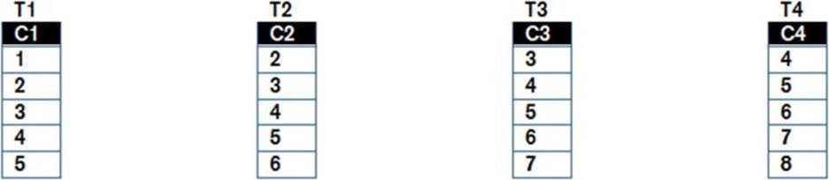
Figure 1-1. The data in our test tables

Left Outer Joins

Listing 1-22 provides the first outer join example. It shows a left outer join. Such a join makes rows from the second table, the table on the right-hand side, optional. You’ll get all relevant rows from the table on the left-hand side regardless of corresponding rows in the right-hand side of the table.

Listing 1-22. A two table left outer join

SELECT *
FROM t1 LEFT OUTER JOIN t2 ON t1.c1 = t2.c2 AND t1.c1 > 4
WHERE t1.c1 > 3
ORDER BY t1.c1;

C1 C2
---------- ----------
4
5 5

As you can see, the format of the FROM clause is now quite different, and I’ll come back to this. The left operand of the join is called the preserved row source and the right operand the optional row source.

What this query (logically) says is:

· Identify combinations of rows in T1 and T2 that match the criteria T1.C1 = T2.C2 AND T1.C1 > 4.

· For all rows in T1 that do not match any rows in T2, output them with NULL for the columns in T2.

· Eliminate all rows from the result set that do not match the criteria T1.C1 > 3.

· Order the result by T1.C1.

Notice that there is a big difference between a selection predicate and a join predicate. The selection predicate T1.C1 > 3 resulted in the elimination of rows from the result set, but the join predicate T1.C1 > 4 just resulted in the loss of column values from T2.

Not only is there now a big difference between a join predicate and a selection predicate, but the CBO doesn’t have complete freedom to reorder joins. Consider Listing 1-23 that joins all four tables.

Listing 1-23. Four table outer join

SELECT c1
,c2
,c3
,c4
FROM (t3 LEFT JOIN t4 ON t3.c3 = t4.c4)
LEFT JOIN (t2 LEFT JOIN t1 ON t1.c1 = t2.c2) ON t2.c2 = t3.c3
ORDER BY c3;

C1 C2 C3 C4
---------- ---------- ---------- ----------
3 3 3
4 4 4 4
5 5 5 5
6 6 6
7 7

To make things a little clearer, I have added optional parentheses so you can see the intention. Notice also that the keyword OUTER is optional and I have omitted it here.

With one special exception, which I’ll come to when I discuss hash input swapping later, the CBO always uses the left operand of the left outer join (the preserved row source) as the driving row source in the join. Therefore, the CBO has limited choice in which join order to use here. The join order that was specified was ((T3 T4) (T2 T1)).

The CBO did, in fact, have a choice of five join orders. All the predicates mandate that:

· T3 precedes T4 in the join order

· T2 precedes T1 in the join order

· T3 precedes T2 in the join order

As an example, Listing 1-24 rewrites Listing 1-23 using the order (((T3 T2) T1) T4) to get the same results.

Listing 1-24. An alternative construction of Listing 1-23

SELECT c1
,c2
,c3
,c4
FROM t3
LEFT JOIN t2 ON t3.c3 = t2.c2
LEFT JOIN t1 ON t2.c2 = t1.c1
LEFT JOIN t4 ON t3.c3 = t4.c4
ORDER BY c3;

Because outer joins had not yet been conceived when SQL was first invented, the traditional syntax has no provision for separating join conditions from selection conditions or for differentiating preserved from optional row sources.

Oracle was an early implementer of outer joins and it devised a proprietary extension to the traditional syntax to denote outer join conditions. The syntax involves modifying the WHERE clause by appending columns from the optional row source with (+) in join conditions. Listing 1-25rewrites Listing 1-24 using the proprietary syntax.

Listing 1-25. Rewrite of Listing 1-24 using proprietary syntax

SELECT c1
,c2
,c3
,c4
FROM t1
,t2
,t3
,t4
WHERE t3.c3 = t2.c2(+) AND t2.c2 = t1.c1(+) AND t3.c3 = t4.c4(+)
ORDER BY c3;

This notation is severely limited in its ability:

· Prior to Oracle Database 12cR1, a table can be the optional row source in at most one join.

· Full and partitioned outer joins, which I’ll discuss shortly, are not supported.

Because of these restrictions, the queries in Listings 1-28, 1-29 and 1-30 can’t be expressed in proprietary syntax. To implement these queries with proprietary syntax, you would need to use factored subqueries, inline views or set operators.

Personally I find this proprietary syntax difficult to read, and this is another reason why I generally advise against its use. You could, however, see this notation in execution plans in the predicate section, which will be discussed in Chapter 8.

The new syntax has been endorsed by the ANSI and is usually referred to as ANSI join syntax. This syntax is supported by all major database vendors and supports inner joins as well. Listing 1-26 shows how to specify an inner join with ANSI syntax.

Listing 1-26. ANSI join syntax with inner joins

SELECT *
FROM t1
LEFT JOIN t2
ON t1.c1 = t2.c2
JOIN t3
ON t2.c2 = t3.c3
CROSS JOIN t4;

C1 C2 C3 C4
---------- ---------- ---------- ----------
3 3 3 4
3 3 3 5
3 3 3 6
3 3 3 7
3 3 3 8
4 4 4 4
4 4 4 5
4 4 4 6
4 4 4 7
4 4 4 8
5 5 5 4
5 5 5 5
5 5 5 6
5 5 5 7
5 5 5 8

The join with T3 is an inner join (you can explicitly add the keyword INNER if you want), and the join with T4 is a Cartesian join; ANSI uses the keywords CROSS JOIN to denote a Cartesian join.

Right Outer Joins

A right outer join is just syntactic sugar. A right outer join preserves rows on the right instead of the left. Listing 1-27 shows how difficult queries can be to read without the right outer join syntax.

Listing 1-27. Complex query without right outer join

SELECT c1, c2, c3
FROM t1
LEFT JOIN
t2
LEFT JOIN
t3
ON t2.c2 = t3.c3
ON t1.c1 = t3.c3
ORDER BY c1;

Listing 1-27 specifies the join order (T1 (T2 T3)). Listing 1-28 shows how to specify the same join order using a right outer join.

Listing 1-28. Right outer join

SELECT c1, c2, c3
FROM t2
LEFT JOIN t3
ON t2.c2 = t3.c3
RIGHT JOIN t1
ON t1.c1 = t3.c3
ORDER BY c1;

Personally, I find the latter syntax easier to read, but it makes no difference to either the execution plan or the results.

Full Outer Joins

As you might guess, a full outer join preserves rows on both sides of the keywords. Listing 1-29 is an example.

Listing 1-29. Full outer join

SELECT *
FROM t1 FULL JOIN t2 ON t1.c1 = t2.c2
ORDER BY t1.c1;

C1 C2
---------- ----------
1
2 2
3 3
4 4
5 5
6

Partitioned Outer Joins

Both left and right outer joins can be partitioned. This term is somewhat overused. To be clear, its use here has nothing to do with the partitioning option, which relates to a physical database design feature.

To explain partitioned outer joins, I will use the SALES table from the SH example schema. To keep the result set small, I am just looking at sales made to countries in Europe between 1998 and 1999. For each year, I want to know the total sold per country vs. the average number of sales per country made to customers born in 1976. Listing 1-30 is my first attempt.

Listing 1-30. First attempt at average sales query

WITH sales_q
AS (SELECT s.*, EXTRACT (YEAR FROM time_id) sale_year
FROM sh.sales s)
SELECT sale_year
,country_name
,NVL (SUM (amount_sold), 0) amount_sold
,AVG (NVL (SUM (amount_sold), 0)) OVER (PARTITION BY sale_year)
avg_sold
FROM sales_q s
JOIN sh.customers c USING (cust_id) -- PARTITION BY (sale_year)
RIGHT JOIN sh.countries co
ON c.country_id = co.country_id AND cust_year_of_birth = 1976
WHERE (sale_year IN (1998, 1999) OR sale_year IS NULL)
AND country_region = 'Europe'
GROUP BY sale_year, country_name
ORDER BY 1, 2;

I begin with a factored subquery to obtain the year of the sale once for convenience. I know that some countries might not have any sales to customers born in 1976, so I have used an outer join on countries and added the CUST_YEAR_OF_BIRTH = 1976 to the join condition rather than the WHERE clause. Notice also the use of the USING clause. This is just shorthand for ON C.CUST_ID = S.CUST_ID. Here are the results:

SALE_YEAR COUNTRY_NAME AMOUNT_SOLD AVG_SOLD
---------- ---------------------------------------- ----------- ----------
1998 Denmark 2359.6 11492.5683
1998 France 28430.27 11492.5683
1998 Germany 6019.98 11492.5683
1998 Italy 5736.7 11492.5683
1998 Spain 15864.76 11492.5683
1998 United Kingdom 10544.1 11492.5683
1999 Denmark 13250.2 21676.8267
1999 France 46967.8 21676.8267
1999 Italy 28545.46 21676.8267
1999 Poland 4251.68 21676.8267
1999 Spain 21503.07 21676.8267
1999 United Kingdom 15542.75 21676.8267
Ireland 0 0
The Netherlands 0 0
Turkey 0 0

The AVG_SOLD column is supposed to contain the average sales for countries in that year and thus is the same for all countries in any year. It is calculated using what is known as an analytic function, which I’ll explain in detail in Chapter 7. You can see that three countries made no qualifying sales and the outer join has added rows for these at the end. But notice that the SALE_YEAR is NULL. That is why I added the OR SALE_YEAR IS NULL clause. It is a debugging aid. Also, Poland made no sales in 1998 and Germany made no sales in 1999. The averages reported are thus incorrect, dividing the total by the six countries that made sales in that year rather than the ten countries in Europe. What you want is to preserve not just every country but every combination of country and year. You can do this by uncommenting the highlightedPARTITION BY clause, as shown in Listing 1-30. This gives the following, more meaningful, results:

SALE_YEAR COUNTRY_NAME AMOUNT_SOLD AVG_SOLD
---------- ---------------------------------------- ----------- ----------
1998 Denmark 2359.6 6895.541
1998 France 28430.27 6895.541
1998 Germany 6019.98 6895.541
1998 Ireland 0 6895.541
1998 Italy 5736.7 6895.541
1998 Poland 0 6895.541
1998 Spain 15864.76 6895.541
1998 The Netherlands 0 6895.541
1998 Turkey 0 6895.541
1998 United Kingdom 10544.1 6895.541
1999 Denmark 13250.2 13006.096
1999 France 46967.8 13006.096
1999 Germany 0 13006.096
1999 Ireland 0 13006.096
1999 Italy 28545.46 13006.096
1999 Poland 4251.68 13006.096
1999 Spain 21503.07 13006.096
1999 The Netherlands 0 13006.096
1999 Turkey 0 13006.096
1999 United Kingdom 15542.75 13006.096

That’s more like it! There are ten rows per year now, one for each country regardless of the sales in that year.

The problem that partitioned outer joins solves is known as data densification. This isn’t always a sensible thing to do, and I’ll return to this issue in Chapter 19.

Note Although partitioned full outer joins are not supported, it is possible to partition the preserved row source instead of the optional row source, as in the example. I can’t think of why you might want to do this, and I can’t find any examples on the Internet of its use.

Summary

This chapter has discussed a few features of SQL that, despite being crucial to optimization, are often overlooked. The main messages I want to leave you with at the end of this chapter are:

· The array interface is crucial for shipping large volumes of data in and out of the database.

· Outer joins limit the opportunity for the CBO to reorder joins.

· Understanding SQL is crucial and making it readable with factored subqueries is an easy way to do this.

I have briefly mentioned the role of the CBO in this chapter and in Chapter 2 I give a more detailed overview of what it does and how it does it.