Expert Oracle SQL: Optimization, Deployment, and Statistics (2014)
PART 2. Advanced Concepts
CHAPTER 7. Advanced SQL Concepts
In this chapter we return to the vagaries of the SQL language to investigate three more of the key concepts that can get you both into a performance jam and out of one.
· The first thing I want to look at is the syntax of query blocks and subqueries. The focus of the discussion is the difference between the way that the CBO treats the two constructs and the way that the SQL Language Reference manual does—a critical issue when we come to analyze execution plans in depth, as we will do in the next chapter.
· The second topic of the chapter is the different types of SQL function. Analytic functions in particular can be really helpful when used correctly and really harmful to performance when used incorrectly.
· The third and final topic in this chapter is the MODEL clause. Many people will go through their whole careers without ever needing to learn what the MODEL clause is or what it does. However, if you, like me, find yourself in desperate need of the MODEL clause you need to recognize when to dive for the Data Warehousing Guide!
Query Blocks and Subqueries
For the Oracle performance specialist the concept of a query block is very important as it is a fundamental processing unit for the CBO and the runtime engine. However, before we can discuss how query blocks work we need to clear up some terminology.
Terminology
The formal definition of a query block in the SQL Language Reference manual is quite complex, but, informally, a query block can be explained quite straightforwardly as “stuff that follows the keyword SELECT.”. The same manual defines a subquery, for which there are four possible constructs:
· A query block
· A query block followed by an ORDER BY clause
· A number of query blocks connected by set operators
· A number of query blocks connected by set operators followed by an ORDER BY clause
The set operators are UNION, UNION ALL, INTERSECT, and MINUS.
![]() Note I have explained the concept of a subquery a little differently than the SQL Language Reference manual did to emphasize that it is illegal for the operands of a set operator to include an ORDER BY clause.
Note I have explained the concept of a subquery a little differently than the SQL Language Reference manual did to emphasize that it is illegal for the operands of a set operator to include an ORDER BY clause.
It turns out that the CBO seems to treat all subqueries as query blocks. It does so as follows:
· A subquery involving set operators is considered as a special type of query block that I will refer to as a set query block.
· An ORDER BY clause is considered part of the query block that it follows.
From now on when I use of the term “query block” in this book the CBO’s interpretation should be assumed; when I use the term “subquery” I will mean it in the normal informal way, namely a query block other than the main query block in a SELECT statement.
How Query Blocks are Processed
Following the SELECT keyword, a query block is written in the following order:
· The optional DISTINCT or UNIQUE operation
· The select list
· Everything else except the ORDER BY clause
· The optional ORDER BY clause
The logical order in which a query block is executed, however, is different:
· Everything else
· The select list
· The optional DISTINCT or UNIQUE operation
· The optional ORDER BY clause
The good news is that with very few exceptions the order in which the various bits and bobs that I have loosely referred to as “everything else” are logically processed in the order in which they appear. In particular, the following clauses, some of which are optional, are written in the same order as they are logically processed:
· The FROM clause
· The WHERE clause
· The GROUP BY clause
· The HAVING clause
· The MODEL clause
Of course, the CBO is free to change the order in which it asks the runtime engine to do things as long as the resulting set of rows is the same as the logical order.
Functions
If your application has been built so that most of your business logic has been implemented outside of the database then you may make very little use of functions in your SQL. However, most commercial and scientific SQL statements are riddled with function calls. The use and abuse of these function calls often results in a huge amount of processing, particularly sorting and aggregation; it is not uncommon for this overhead to dwarf the traditional database overhead of accessing and joining tables. So in this section I want to make sure we all have a clear understanding of how the main function categories work.
The SQL Language Reference manual defines the following function categories:
· Single-row functions
· Aggregate functions
· Analytic functions
· Object reference functions
· Model functions
· OLAP functions
· Data cartridge functions
This section focusses on single-row functions, aggregate functions, and analytic functions. Let us start with aggregate functions.
![]() Note Throughout this section I will be using built-in functions for my examples, but it is important to understand that you can write your own scalar, aggregate, or analytic functions and the same principles that I am about to discuss will apply.
Note Throughout this section I will be using built-in functions for my examples, but it is important to understand that you can write your own scalar, aggregate, or analytic functions and the same principles that I am about to discuss will apply.
Aggregate Functions
Some of the readers of this book will feel fairly fluent with aggregate functions, but I think it is important to review the concepts formally so that there is no confusion when we come to looking at analytic functions and the MODEL clause shortly.
The Concept of Aggregation
Simply put, aggregation involves taking a set of items, producing a single value, and then discarding the input. Listing 7-1 shows the two different ways that aggregation can be triggered.
Listing 7-1. The use of GROUP BY and analytic functions to trigger aggregation
CREATE TABLE t1
AS
SELECT DATE '2013-12-31' + ROWNUM transaction_date
,MOD (ROWNUM, 4) + 1 channel_id
,MOD (ROWNUM, 5) + 1 cust_id
,DECODE (ROWNUM
,1, 4
,ROWNUM * ROWNUM + DECODE (MOD (ROWNUM, 7), 3, 3000, 0))
sales_amount
FROM DUAL
CONNECT BY LEVEL <= 100;
-- No Aggregation in next query
SELECT * FROM t1;
--Exactly one row returned in next query
SELECT COUNT (*) cnt FROM t1;
-- 0 or more rows returned in next query
SELECT channel_id
FROM t1
GROUP BY channel_id;
-- At most one row returned in next query
SELECT 1 non_empty_flag
FROM t1
HAVING COUNT (*) > 0;
-- 0 or more rows returned in next query
SELECT channel_id, COUNT (*) cnt
FROM t1
GROUP BY channel_id
HAVING COUNT (*) < 2;
Listing 7-1 includes create a table T1 and then issues several queries.
· The first query in Listing 7-1 contains no aggregate function and no GROUP BY clause so no aggregation occurs.
· The second query includes the COUNT (*) aggregate function. Since no GROUP BY clause is specified the whole table is aggregated and exactly one row is returned. To be clear, if T1 were empty the query would still return one row and the value of CNT would be 0.
· The third query includes a GROUP BY clause, and so even though no aggregate function appears in the statement, aggregation still takes place. A GROUP BY operator returns one row for every distinct value of the expressions specified in the GROUP BY clause. So in this case there would be one row for each distinct value of CHANNEL_ID, and when the table is empty no rows are returned.
· The fourth query in Listing 7-1 shows that an aggregate function doesn’t need to be placed in the select list to trigger aggregation. The HAVING clause applies a filter after aggregation, unlike a WHERE clause that filters before aggregation. So in this case if T1 were empty the value of COUNT (*) would be 0 and the query would return 0 rows. If there are rows in the table the query would return one row.
· Of course, the most common way aggregation is used is with the GROUP BY clause and aggregate functions used together. The GROUP BY clause in the final query in Listing 7-1 ensures that only values of CHANNEL_ID that occur at least once in T1 are returned, so it is not possible for CNT to have a value of 0. The HAVING clause removes any rows where COUNT (*) >= 2, so if this final query returns any rows the value of CNT will be 1 in all cases!
Sorting Aggregating Functions
Many aggregate functions require a sort to operate effectively. Listing 7-2 shows how the MEDIAN aggregate function might be used.
Listing 7-2. Use of a sorting aggregate function
SELECT channel_id, MEDIAN (sales_amount) med, COUNT (*) cnt
FROM t1
GROUP BY channel_id;
----------------------------
| Id | Operation |
----------------------------
| 0 | SELECT STATEMENT |
| 1 | SORT GROUP BY |
| 2 | TABLE ACCESS FULL|
----------------------------
![]() Note The median of an odd number of numbers is the middle one in the sorted list. For an even number of values it is the average (mean) of the two middle numbers. So the median of 2, 4, 6, 8, 100 and 102 is 7 (the average of 6 and 8).
Note The median of an odd number of numbers is the middle one in the sorted list. For an even number of values it is the average (mean) of the two middle numbers. So the median of 2, 4, 6, 8, 100 and 102 is 7 (the average of 6 and 8).
From Listing 7-2 on I will be showing the execution plans for SQL statements in the format produced by DBMS_XPLAN.DISPLAY without using the EXPLAIN PLAN statement and without showing explicit calls to the DBMS_XPLAN.DISPLAY function. Furthermore, I will only be showing the relevant portions of the execution plan. These measures are purely to save space. The downloadable materials are not abbreviated in this way.
Listing 7-2 aggregates the 100 rows in the table T1 we created in Listing 7-1 to return four rows, one for each distinct value of CHANNEL_ID. The value of MED in these rows represents the median of the 25 rows in each group. The basic execution plan for this statement is also shown inListing 7-2, and operation 1 is the sort used to implement this.
![]() Note If the truth be known, there are actually six sorts performed in Listing 7-2! The first sort is by C1 to create the four groups. Then each group is sorted by SALES_AMOUNT as required by the MEDIAN function. If you examine the statistic “sorts (rows)” before and after the query inListing 7-2 you will see that it increases by 200, twice the number in the table; each row is sorted twice. And if multiple aggregate functions with different sort orders are used, then each group may be sorted multiple times.
Note If the truth be known, there are actually six sorts performed in Listing 7-2! The first sort is by C1 to create the four groups. Then each group is sorted by SALES_AMOUNT as required by the MEDIAN function. If you examine the statistic “sorts (rows)” before and after the query inListing 7-2 you will see that it increases by 200, twice the number in the table; each row is sorted twice. And if multiple aggregate functions with different sort orders are used, then each group may be sorted multiple times.
The code that you can use to examine the statistic is:
SELECT VALUE FROM v$mystat NATURAL JOIN v$statname WHERE name = 'sorts (rows)';
Non-sorting Aggregating Functions
Not all aggregate functions require a sort. I use the term “non-sorting aggregate functions” (NSAFs) to refer to aggregate functions that require no sort. An example of an NSAF is COUNT. COUNT doesn’t need to sort: as each row is processed COUNT simply increments a running tally. Other NSAFs, like SUM, AVG, and STDDEV are also implemented by keeping running tallies of one form or another.
When an NSAF and a GROUP BY clause both appear in a query block then the NSAF needs to keep running tallies for each group. Oracle database 10g introduced a feature called hash aggregation that allows NSAFs to find the tallies for each group by a lookup in a hash table rather than a lookup from a sorted list. Let us have a look at Listing 7-3, which shows the feature in action.
Listing 7-3. Hash aggregation for NSAFs
SELECT channel_id
,AVG (sales_amount)
,SUM (sales_amount)
,STDDEV (sales_amount)
,COUNT (*)
FROM t1
GROUP BY channel_id;
------------------------------------
| Id | Operation | Name |
------------------------------------
| 0 | SELECT STATEMENT | |
| 1 | HASH GROUP BY | |
| 2 | TABLE ACCESS FULL| T1 |
------------------------------------
Hash aggregation requires that all aggregate functions used in the query block are NSAFs; all of the functions in Listing 7-3 are NSAFs, so the operation HASH GROUP BY is used to avoid any sorting.
![]() Note Not all NSAFs can take advantage of hash aggregation. Those that can’t include COLLECT, FIRST, LAST, RANK, SYS_XMLAGG, and XMLAGG. These functions use the SORT GROUP BY operation when a GROUP BY clause is used and the non-sorting SORT AGGREGATEoperation when no GROUP BY clause is specified. This restriction is presumably due to the variable size of the aggregated values.
Note Not all NSAFs can take advantage of hash aggregation. Those that can’t include COLLECT, FIRST, LAST, RANK, SYS_XMLAGG, and XMLAGG. These functions use the SORT GROUP BY operation when a GROUP BY clause is used and the non-sorting SORT AGGREGATEoperation when no GROUP BY clause is specified. This restriction is presumably due to the variable size of the aggregated values.
Just because the CBO can use hash aggregation doesn’t mean that it will. Hash aggregation will not be used when the data being grouped is already sorted or needs to be sorted anyway. Listing 7-4 provides two examples.
Listing 7-4. SORT GROUP BY with NSAFs
SELECT channel_id, AVG (sales_amount) mean
FROM t1
WHERE channel_id IS NOT NULL
GROUP BY channel_id
ORDER BY channel_id;
CREATE INDEX t1_i1
ON t1 (channel_id);
SELECT channel_id, AVG (sales_amount) mean
FROM t1
WHERE channel_id IS NOT NULL
GROUP BY channel_id;
DROP INDEX t1_i1;
-----------------------------------
| Id | Operation | Name |
-----------------------------------
| 0 | SELECT STATEMENT | |
| 1 | SORT GROUP BY | |
|* 2 | TABLE ACCESS FULL| T1 |
-----------------------------------
----------------------------------------------
| Id | Operation | Name |
----------------------------------------------
| 0 | SELECT STATEMENT | |
| 1 | SORT GROUP BY NOSORT | |
| 2 | TABLE ACCESS BY INDEX ROWID| T1 |
|* 3 | INDEX FULL SCAN | T1_I1 |
----------------------------------------------
The first query in Listing 7-4 includes an ORDER BY clause. In this case there is no getting around a sort so hash aggregation gains nothing.
![]() Note You might think that it would be more efficient to perform hash aggregation and then sort the aggregated rows. After all, if you have 1,000,000 rows and 10 groups wouldn’t it be better to sort the 10 aggregated rows rather than the 1,000,000 un-aggregated ones? In fact, in such a case only 10 rows would be kept in the sort work area; the NSAFs would just keep their running tallies for each group as with hash aggregation.
Note You might think that it would be more efficient to perform hash aggregation and then sort the aggregated rows. After all, if you have 1,000,000 rows and 10 groups wouldn’t it be better to sort the 10 aggregated rows rather than the 1,000,000 un-aggregated ones? In fact, in such a case only 10 rows would be kept in the sort work area; the NSAFs would just keep their running tallies for each group as with hash aggregation.
Before executing the second query in Listing 7-4 we create an index on CHANNEL_ID. The index will return the data in sorted order anyway so we don’t need either an explicit sort or a hash table, and the aggregation is processed for each group in turn. Notice that that the name for operation 1 is now self-contradictory: SORT GROUP BY NOSORT. Of course, no sort takes place.
Analytic Functions
Now that we fully understand what aggregate functions are and how they are processed, it is time to move on to the more complex concept of analytic functions. Analytic functions have the potential to make SQL statements easy to read and perform well. They can also make SQL impenetrable and slow when used incorrectly.
The Concept of Analytics
We said that aggregate functions discard the original rows being aggregated. What happens if that is not what we want? Do you remember Listing 3-1? That query listed each row in SCOTT.EMP together with aggregated data about that employee’s department. We used a subquery to accomplish that. Listing 7-5 is another example of the same technique using the table T1 from Listing 7-1 and the COUNT function.
Listing 7-5. Use of subqueries to implement analytics
SELECT outer.*
, (SELECT COUNT (*)
FROM t1 inner
WHERE inner.channel_id = outer.channel_id)
med
FROM t1 outer;
-----------------------------------
| Id | Operation | Name |
-----------------------------------
| 0 | SELECT STATEMENT | |
| 1 | SORT GROUP BY | |
|* 2 | TABLE ACCESS FULL| T1 |
| 3 | TABLE ACCESS FULL | T1 |
-----------------------------------
The query in Listing 7-5 lists the 100 rows in T1 together with an extra column containing the matching count of rows for the corresponding value of CHANNEL_ID. The execution plan for the query seems to suggest that we will perform the subquery for each of the 100 rows in T1. However, as with Listing 3-1, scalar subquery caching will mean that we only perform the subquery four times, one for each distinct value of CHANNEL_ID. Nevertheless, when we add in operation 3 from the main query we will still perform five full table scans of T1 in the course of the query.
Subqueries can also be used to denote ordering. Listing 7-6 shows how we might add a row number and a rank to a sorted list.
Listing 7-6. Numbering output using ROWNUM and subqueries
WITH q1
AS ( SELECT *
FROM t1
ORDER BY transaction_date)
SELECT ROWNUM rn
, (SELECT COUNT (*)+1
FROM q1 inner
WHERE inner.sales_amount < outer.sales_amount)
rank_sales,outer.*
FROM q1 outer
ORDER BY sales_amount;
-- First few rows of output
RN RANK_SALES TRANSACTI CHANNEL_ID CUST_ID SALES_AMOUNT
---------- ---------- --------- ---------- ---------- ------------
1 1 01-JAN-14 2 2 4
2 1 02-JAN-14 3 3 4
4 3 04-JAN-14 1 5 16
5 4 05-JAN-14 2 1 25
------------------------------------------------------------------
| Id | Operation | Name |
------------------------------------------------------------------
| 0 | SELECT STATEMENT | |
| 1 | SORT AGGREGATE | |
|* 2 | VIEW | |
| 3 | TABLE ACCESS FULL | SYS_TEMP_0FD9D664B_479D89AC |
| 4 | TEMP TABLE TRANSFORMATION | |
| 5 | LOAD AS SELECT | SYS_TEMP_0FD9D664B_479D89AC |
| 6 | SORT ORDER BY | |
| 7 | TABLE ACCESS FULL | T1 |
| 8 | SORT ORDER BY | |
| 9 | COUNT | |
| 10 | VIEW | |
| 11 | TABLE ACCESS FULL | SYS_TEMP_0FD9D664B_479D89AC |
------------------------------------------------------------------
The factored subquery Q1 in Listing 7-6 orders the rows in the table, then we use the ROWNUM pseudocolumn to identify the position of each row in the sorted list. The column RANK_SALES differs slightly from RN in that rows with identical sales figures (such as the first two rows) are given equal position. The execution plan for this statement is far from straightforward. There must surely be an easier and more efficient way! Indeed there is; analytic functions offer solutions to many inefficient subqueries.
![]() Note All analytic functions have an equivalent formulation involving subqueries. Sometimes the analytic function performs better than the subquery, and sometimes the subquery performs better than the analytic function.
Note All analytic functions have an equivalent formulation involving subqueries. Sometimes the analytic function performs better than the subquery, and sometimes the subquery performs better than the analytic function.
Aggregate Functions Used as Analytics
Most, but not all, aggregate functions can also be used as analytic functions. Listing 7-7 rewrites Listing 7-5, this time using COUNT as an analytic function rather than an aggregate function.
Listing 7-7. An aggregate function used as an analytic function
SELECT t1.*, COUNT (sales_amount) OVER (PARTITION BY channel_id)cnt FROM t1;
-----------------------------------
| Id | Operation | Name |
-----------------------------------
| 0 | SELECT STATEMENT | |
| 1 | WINDOW SORT | |
| 2 | TABLE ACCESS FULL| T1 |
-----------------------------------
The presence of the OVER clause in Listing 7-7 indicates that the MEDIAN function is being used as an analytic function rather than as an aggregate function. The query returns all 100 rows of T1, and the column CNT is added just as in Listing 7-5. Although the rows returned by Listing 7-5 and Listing 7-7 are the same, the way the queries execute are quite different, and the rows will likely be returned in a different order.
The execution plan shown in Listing 7-7 includes the WINDOW SORT operation that is specific to analytic functions. Unlike the SORT GROUP BY operation that may make several sorts, the WINDOW SORT operation performs just one sort of the rows it receives from its child. In the case of Listing 7-7 the rows are sorted by the composite key containing the columns CHANNEL_ID and SALES_AMOUNT, implicitly creating a group for each value of CHANNEL_ID. The COUNT function then processes each group in two phases:
· In the first phase, the group is processed to identify the COUNT for the group as with the aggregate variant of the COUNT function.
· In the second phase, each row from the group is output with the same calculated count being provided as an extra column on each row.
The term PARTITION BY is the analytic equivalent to the GROUP BY clause in aggregation; if the PARTITION BY keywords are omitted then the analytic function processes the entire result set.
Listing 7-8 shows a simple analytic that processes the entire result set.
Listing 7-8. Use of a NSAF in an analytic
SELECT t1.*, AVG (sales_amount) OVER ()average_sales_amount FROM t1;
-----------------------------------
| Id | Operation | Name |
-----------------------------------
| 0 | SELECT STATEMENT | |
| 1 | WINDOW BUFFER | |
| 2 | TABLE ACCESS FULL| T1 |
-----------------------------------
The query in Listing 7-8 adds a column, AVERAGE_SALES_AMOUNT, that has the same value for all 100 rows in T1. That value is the average value of SALES_AMOUNT for the entire table. Notice that because AVG is an NSAF and there is no PARTITION BY clause there is no need to sort at all. As a consequence the WINDOW BUFFER operation is used instead of WINDOW SORT.
As with aggregation, when multiple functions are used multiple sorts may be needed. In the case of analytics, however, each sort has its own operation. Look at the difference in the execution plans for the two queries in Listing 7-9.
Listing 7-9. Comparison of multiple sorts with aggregation and analytics
SELECT MEDIAN (channel_id) med_channel_id
,MEDIAN (sales_amount) med_sales_amount
FROM t1;
-----------------------------------
| Id | Operation | Name |
-----------------------------------
| 0 | SELECT STATEMENT | |
| 1 | SORT GROUP BY | |
| 2 | TABLE ACCESS FULL| T1 |
-----------------------------------
SELECT t1.*
,MEDIAN (channel_id) OVER ()med_channel_id
,MEDIAN (sales_amount) OVER ()med_sales_amount
FROM t1;
-----------------------------
| Id | Operation |
-----------------------------
| 0 | SELECT STATEMENT |
| 1 | WINDOW SORT |
| 2 | WINDOW SORT |
| 3 | TABLE ACCESS FULL|
-----------------------------
The first query in Listing 7-9 returns one row with the median values of CHANNEL_ID and SALES_AMOUNT. Each aggregate function call requires its own sort: the first a sort by CHANNEL_ID and the second a sort by SALES_AMOUNT. However, that detail is masked by the SORT GROUP BY operation. The second query involves analytic function calls and returns all 100 rows in T1. This second query also requires two sorts. In this case, however, the two sorts each have their own WINDOW SORT operation in the execution plan.
Analytic-only Functions
Although nearly all aggregate functions can operate as analytic functions, there are a lot of analytic functions that have no aggregate counterpart. By way of an example, Listing 7-10 rewrites Listing 7-6 in a way that is both easier to read and more efficient.
Listing 7-10. Introducing the ROW_NUMBER and RANK analytic functions
SELECT ROW_NUMBER () OVER (ORDER BY sales_amount) rn
,RANK () OVER (ORDER BY sales_amount) rank_sales
,t1.*
FROM t1
ORDER BY sales_amount;
----------------------------
| Id | Operation |
----------------------------
| 0 | SELECT STATEMENT |
| 1 | WINDOW SORT |
| 2 | TABLE ACCESS FULL|
----------------------------
The output of the query in Listing 7-10 is identical to that in 7-6. The WINDOW SORT operation sorts the rows by SALES_AMOUNT, and then the ROW_NUMBER analytic function reads the rows from the sorted buffer and adds the additional column indicating the position in the list. TheRANK function is similar to ROW_NUMBER except that rows with equal values of SALES_AMOUNT are given the same ranking. Notice that the ORDER BY clause causes no additional overhead as the data is already sorted. But this behavior is not guaranteed, and in case the CBO does something different in future releases it is best to add the ORDER BY clause if the ordering is important.
Analytic Sub-clauses
We have seen that analytic functions include the keyword OVER followed by a pair of parentheses. Inside these parentheses there are up to three optional sub-clauses. These are the query partition sub-clause, the order by sub-clause, and the windowing sub-clause. If more than one of these sub-clauses are present then they must be written in the prescribed order. Let us look at each of these sub-clauses in more detail.
Query Partition Sub-clause
This sub-clause uses the keywords PARTITION BY to separate the rows into groups and then runs the analytic function on each group independently.
![]() Note The keywords PARTITION BY when used in analytic functions have nothing to do with the licensed feature that permits indexes and tables to be split into multiple segments. Nor is there any relationship between the term PARTITION BY in analytics and the partitioned outer-join concept that we discussed in Chapter 1.
Note The keywords PARTITION BY when used in analytic functions have nothing to do with the licensed feature that permits indexes and tables to be split into multiple segments. Nor is there any relationship between the term PARTITION BY in analytics and the partitioned outer-join concept that we discussed in Chapter 1.
We have seen an example of the query partition sub-clause in Listing 7-7. Listing 7-11 provides us with another example that is a slight modification of Listing 7-8.
Listing 7-11. NSAF analytic with a PARTITION BY clause
SELECT t1.*
,AVG (sales_amount) OVER (PARTITION BY channel_id) average_sales_amount
FROM t1;
----------------------------
| Id | Operation |
----------------------------
| 0 | SELECT STATEMENT |
| 1 | WINDOW SORT |
| 2 | TABLE ACCESS FULL|
----------------------------
The only difference between the query in Listing 7-8 and the query in Listing 7-11 is the addition of the query partition clause. So in Listing 7-8 the value of AVERAGE_SALES_AMOUNT for the row where CHANNEL_ID is 1 and SALES_AMOUNT is 16 is 3803.53, as it is for every row. The average value of SALES_AMOUNT of all 100 rows in T1 is 3803.53. On the other hand, the query containing the PARTITION BY clause returns a value of 3896 for AVERAGE_SALES_AMOUNT when CHANNEL_ID is 1 and SALES_AMOUNT is 16. This is the average of the 25 rows where CHANNEL_ID is 1.
You will notice that the execution plan in Listing 7-11 differs from that in Listing 7-8. The query partition clause in Listing 7-11 requires the rows to be sorted by CHANNEL_ID even though the AVG function is an NSAF.
ORDER BY Sub-clause
When the MEDIAN function is used as an analytic function the order in which the rows are sorted is determined by the argument to the MEDIAN function, and in this case the order by sub-clause would be redundant and is illegal. However, we have already seen an example of a legal use of the order by sub-clause in Listing 7-10 that introduced the ROW_NUMBER analytic function. Listing 7-12 shows another use of the order by sub-clause.
Listing 7-12. The NTILE analytic function
SELECT t1.*, NTILE (4) OVER (ORDER BY sales_amount) nt FROM t1;
The query in Listing 7-12 sorts the 100 rows in T1 by SALES_AMOUNT. The execution plan for this statement appears to be the same as those in Listing 7-10 and 7-11 so I haven’t shown it again. The NTILE function identifies percentiles, and its argument indicates how many. In this case the function returns 1 for the 25 rows in the lowest quartile (the rows with the lowest value of SALES_AMOUNT), 2 for the 25 rows in the second quartile, 3 for the 25 rows in the third quartile, and 4 for the 25 rows with the highest values for SALES_AMOUNT.
It is possible to combine the query partition clause and the order by clause in the same function call. Listing 7-13 shows how this is done and introduces a new analytic function at the same time.
Listing 7-13. The LAG analytic functions
SELECT t1.*
,LAG (sales_amount)
OVER (PARTITION BY channel_id, cust_id ORDER BY transaction_date)
prev_sales_amount
FROM t1
ORDER BY channel_id, sales_amount;
The LAG function picks the value of an expression from an earlier row. The function takes three arguments.
· The first, mandatory, argument is the column or expression to pick
· The second, optional, argument is the number of rows back to go and defaults to 1, in other words the preceding row
· The third and final optional argument is the value returned if the offset goes beyond the scope of the window. If you do not specify the third argument then it defaults to NULL.
This call to the LAG function operates by logically grouping the 100 rows into 20 groups of 5 rows based on the distinct values of CHANNEL_ID and CUST_ID. Within each group we take the value of SALES_AMOUNT from the preceding row when ordered by TRANSACTION_DATE. In other words, we see the details of a transaction together with the SALES_AMOUNT from the previous transaction made by the same customer using the same channel. Listing 7-14 shows a few sample rows from the output.
Listing 7-14. Sample output from Listing 7-13
TRANSACTION_DATE CHANNEL_ID CUST_ID SALES_AMOUNT PREV_SALES_AMOUNT
20/01/2014 1 1 400
09/02/2014 1 1 1600 400
01/03/2014 1 1 3600 1600
21/03/2014 1 1 9400 3600
10/04/2014 1 1 10000 9400
16/01/2014 1 2 256
Notice that the highlighted rows are the first in their group. In this case, LAG returns NULL because we didn’t specify three arguments to the function. You should know that there is a LEAD function call as well. This takes values from a succeeding, rather than preceding, row.
![]() Note A call to LEAD with a descending sort order yields the same value as a call to LAG with an ascending sort order and vice versa. Only the order of the rows returned by the WINDOW SORT operation changes.
Note A call to LEAD with a descending sort order yields the same value as a call to LAG with an ascending sort order and vice versa. Only the order of the rows returned by the WINDOW SORT operation changes.
Windowing Analytic Sub-clause
The windowing sub-clause is the most complex of the three types of sub-clause but also one of the most useful. The rules for its use are quite complex, and I can only provide an introduction here.
· A windowing sub-clause is only allowed for a subset of NSAFs.
· If a windowing sub-clause is specified, an order by sub-clause is also required.
· For those functions that support a windowing sub-clause a default window sub-clause is implied if an order by sub-clause is provided.
Like the query partition clause, the windowing clause restricts the analytic function to a subset of rows, but unlike the query partition clause the range is dynamic. Consider Listing 7-15, which shows the windowing clause in action.
Listing 7-15. An implementation of a moving average
SELECT t1.*
,AVG (
sales_amount)
OVER (PARTITION BY cust_id
ORDER BY transaction_date
ROWS BETWEEN 2 PRECEDING AND CURRENT ROW)
mov_avg
FROM t1;
-- Sample output
TRANSACTION_DATE CHANNEL_ID CUST_ID SALES_AMOUNT MOV_AVG
05-JAN-14 2 1 25 25
10-JAN-14 3 1 3100 1562.5
15-JAN-14 4 1 225 1116.66666666667
20-JAN-14 1 1 400 1241.66666666667
Listing 7-15 implements a traditional moving-average calculation, including the current row and the two that precede it, assuming that they exist. The value returned by the function is the average SALES_AMOUNT of the last three transactions with that customer. The sample output shows some rows where CUST_ID is 1. The first row has a window of one row, the second provides the average of the first two rows, and the third and subsequent rows in the group average three numbers. So the fourth row provides an average of 3100, 225, and 400, which is 1241⅔.
The default windowing specification is ROWS BETWEEN UNBOUNDED PRECEDING AND CURRENT ROW, and one very common use of this is to implement a running total, as shown in Listing 7-16.
Listing 7-16. A running total using SUM with an implied windowing sub-clause
SELECT t1.*
,SUM (sales_amount)
OVER (PARTITION BY cust_id ORDER BY transaction_date)
moving_balance
FROM t1;
-- Sample output (first few rows)
TRANSACTION_DATE CHANNEL_ID CUST_ID SALES_AMOUNT MOVING_BALANCE
05-JAN-14 2 1 25 25
10-JAN-14 3 1 3100 3125
15-JAN-14 4 1 225 3350
20-JAN-14 1 1 400 3750
At first glance the order by sub-clause used with the SUM function seems ludicrous because the sum of a set of values is the same no matter how they are ordered. However, because SUM supports windowing the implication of the order by sub-clause is that we are summing just the current and preceding rows; the windowing sub-clause is implied. Do you see how the values of SALES_AMOUNT are accumulated in the MOVING_BALANCE column?
Windowing is also supported for logical ranges. Listing 7-17 shows an example of a logical range.
Listing 7-17. Windowing over a specified time period
SELECT t1.*
,AVG (
sales_amount)
OVER (PARTITION BY cust_id
ORDER BY transaction_date
RANGE INTERVAL '10' DAY PRECEDING)
mov_avg
FROM t1;
The query in Listing 7-17 specifies that transactions made in the eleven days ending on the transaction date of the current row are included in the window. Notice that I have abbreviated the window specification here; by default the window closes on the current row or value. Because of the way the data was setup in T1, the output of Listing 7-17 is identical to that in Listing 7-15.
![]() Note When logical ranges are used the keywords CURRENT ROW, which are implicit in Listing 7-17, really mean current value. So if there were multiple rows with the same value of TRANSACTION_DATE as the current row then the analytic would include the values ofSALES_AMOUNT from all such rows in its average.
Note When logical ranges are used the keywords CURRENT ROW, which are implicit in Listing 7-17, really mean current value. So if there were multiple rows with the same value of TRANSACTION_DATE as the current row then the analytic would include the values ofSALES_AMOUNT from all such rows in its average.
Why Windowing is Restricted to NSAFs
A while ago a client asked me to implement a moving median, much like the moving average in Listing 7-15. I couldn’t use the MEDIAN function with a windowing sub-clause because windowing isn’t supported for the MEDIAN function, as it is inefficient.
To understand why calculating a moving median is so difficult, let us take another look at the sample output shown in Listing 7-15. Before calculating the last MOVING_BALANCE the window has to be “slid” to exclude the first row and include the fourth. The rows included in the resultant window are highlighted. To make this “sliding” activity efficient, the WINDOW SORT operation has sorted the rows by CUST_ID and TRANSACTION_DATE.
Once the rows in the window have been identified, it is then time to invoke the analytic function. For NSAFs, such as AVG used in Listing 7-15, this is a simple matter of scanning the values and keeping track of the tally as usual.
![]() Note For many functions, including AVG, it is theoretically possible to calculate the new values without scanning all the rows in the window each time. However, for functions like MAX and MIN a scan is required.
Note For many functions, including AVG, it is theoretically possible to calculate the new values without scanning all the rows in the window each time. However, for functions like MAX and MIN a scan is required.
Now suppose we wanted to calculate a moving median for SALES_AMOUNT rather than a moving average. The rows in our window are sorted by TRANSACTION_DATE and would have to be re-sorted by SALES_AMOUNT. This re-sort would be required each time the window slides to a new row in T1. The same type of argument can be made for any aggregate function that sorts.
Of course, regardless of the inefficiency of the calculation, my client still had a requirement for a moving median! I’ll come back to how I solved this problem shortly when we discuss the MODEL clause.
Analytics as a Double-edged Sword
These analytics seem really cool. Analytic functions allow us to write succinct and efficient code and impress our friends with our SQL prowess at the same time! What could be better? Quite a lot, actually.
Let me create a new table T2 that shows how analytic functions can lead you into the performance mire more often than they can extract you from it. Listing 7-18 shows a test case similar to the one a naïve Tony Hasler developed a few years ago to demonstrate how super-fast analytic functions were. I was in for a shock!
Listing 7-18. The downside of analytic functions
CREATE TABLE t2
(
c1 NUMBER
,c2 NUMBER
,big_column1 CHAR (2000)
,big_column2 CHAR (2000)
);
INSERT /*+ APPEND */ INTO t2 (c1
,c2
,big_column1
,big_column2)
SELECT ROWNUM
,MOD (ROWNUM, 5)
,RPAD ('X', 2000)
,RPAD ('X', 2000)
FROM DUAL
CONNECT BY LEVEL <= 50000;
COMMIT;
WITH q1
AS ( SELECT c2, AVG (c1) avg_c1
FROM t2
GROUP BY c2)
SELECT *
FROM t2 NATURAL JOIN q1;
-----------------------------------------------------------------------------
| Id | Operation | Name | Rows | Bytes | Cost (%CPU)| Time |
-----------------------------------------------------------------------------
| 0 | SELECT STATEMENT | | 50000 | 192M| 27106 (1)| 00:00:02 |
|* 1 | HASH JOIN | | 50000 | 192M| 27106 (1)| 00:00:02 |
| 2 | VIEW | | 5 | 130 | 13553 (1)| 00:00:01 |
| 3 | HASH GROUP BY | | 5 | 40 | 13553 (1)| 00:00:01 |
| 4 | TABLE ACCESS FULL| T2 | 50000 | 390K| 13552 (1)| 00:00:01 |
| 5 | TABLE ACCESS FULL | T2 | 50000 | 191M| 13552 (1)| 00:00:01 |
-----------------------------------------------------------------------------
Predicate Information (identified by operation id):
---------------------------------------------------
1 - access("T2"."C2"="Q1"."C2")
SELECT t2.*, AVG (c1) OVER (PARTITION BY c2) avg_c1 FROM t2;
-----------------------------------------------------------------------------------
| Id | Operation | Name | Rows | Bytes |TempSpc| Cost (%CPU)| Time |
-----------------------------------------------------------------------------------
| 0 | SELECT STATEMENT | | 50000 | 191M| | 55293 (1)| 00:00:03 |
| 1 | WINDOW SORT | | 50000 | 191M| 195M| 55293 (1)| 00:00:03 |
| 2 | TABLE ACCESS FULL| T2 | 50000 | 191M| | 13552 (1)| 00:00:01 |
-----------------------------------------------------------------------------------
Listing 7-18 creates a test table and then issues two queries that generate precisely the same results. The first query is typical of those from a junior programmer who knows nothing of analytic functions but is keen to show off knowledge of subquery factoring and ANSI syntax. The CBO seems to feel that there will be 5.8 billion rows consuming 21 terabytes of space. All of this horror should surely be avoided.
The second query in Listing 7-18 seems much more efficient. We have eliminated that “offensive” second full table scan of T2. Great—so why is the estimated (and actual) elapsed time for the second higher than for the first?
The clue to the problem lies in the column in the execution plan named “TempSpc” for “Temporary Table Space” that only appears in the execution plan for the second query. The big problem with analytics is that the sort is based on the entire result set. The data aggregated in the hypothetical junior programmer’s SQL excludes BIG_COLUMN1 and BIG_COLUMN2. We can, therefore, aggregate the data in memory, and because AVG is an NSAF we don’t need any sort at all! Unless you have a large enough SGA you are never going to sort the data in the second query in memory, and that disk-based sort will take much longer than an extra full-table scan.
![]() Note The execution plans shown in Listing 17-18 were prepared on a database with a 512Mb SGA. If you try running these examples on a database with a large SGA you may need to increase the number of rows in T2 from 50,000 to a much larger value to see the effect. Similarly, if you find the second query taking too long you may need to reduce the number of rows to a smaller value.
Note The execution plans shown in Listing 17-18 were prepared on a database with a 512Mb SGA. If you try running these examples on a database with a large SGA you may need to increase the number of rows in T2 from 50,000 to a much larger value to see the effect. Similarly, if you find the second query taking too long you may need to reduce the number of rows to a smaller value.
Combining Aggregate and Analytic Functions
Analytic functions are evaluated after any optional aggregation. The first consequence of this fact is that analytic functions cannot appear in a WHERE clause, a GROUP BY clause, or a HAVING clause; analytic functions can only be used with the MODEL clause, as part of a select list, or as part of an expression in an ORDER BY clause. The second consequence of the late point at which analytics are evaluated is that the results of aggregation can be used as inputs to analytic functions. Listing 7-19 gives an example.
Listing 7-19. Combining aggregate and analytic functions
SELECT cust_id
,COUNT (*) tran_count
,SUM (sales_amount) total_sales
,100 * SUM (sales_amount) / SUM (SUM (sales_amount)) OVER ()
pct_revenue1
,100 * ratio_to_report (SUM (sales_amount)) OVER () pct_revenue2
FROM t1
GROUP BY cust_id;
------------------------------------
| Id | Operation | Name |
------------------------------------
| 0 | SELECT STATEMENT | |
| 1 | WINDOW BUFFER | |
| 2 | HASH GROUP BY | |
| 3 | TABLE ACCESS FULL| T1 |
------------------------------------
CUST_ID TRAN_COUNT TOTAL_SALES PCT_REVENUE1 PCT_REVENUE2
1 20 80750 21.2302781889455 21.2302781889455
2 20 69673 18.3179835573796 18.3179835573796
4 20 76630 20.1470739024012 20.1470739024012
5 20 78670 20.6834177724377 20.6834177724377
3 20 74630 19.621246578836 19.621246578836
Listing 7-19 aggregates the 100 rows in T1 into five groups, one for each CUST_ID. We use aggregate functions to calculate TRAN_COUNT, the number of transactions with the customer, and TOTAL_SALES, the sum of SALES_AMOUNT for the customer. As you can see from the execution plan, at that point the result of the hash aggregation in operation 2 is passed to the WINDOW BUFFER operation that supports the un-partitioned NSAF analytic function calls.
The last two columns, PCT_REVENUE1 and PCT_REVENUE2, show the percentage of revenue that the customer contributed. Although the values of the two columns are the same, the calculations are performed slightly differently. PCT_REVENUE1 is evaluated by dividing the aggregated sum of SALES_AMOUNT for the customer by the sum of all aggregated sales for all customers. PCT_REVENUE2 makes use of a special analytic function RATIO_TO_REPORT that makes it easier to write such expressions.
I think that some people may find this sort of SQL difficult to read, and I don’t suggest that you consider Listing 7-19 good coding practice. A slightly lengthier, but clearer, way to write the SQL in Listing 7-19 is shown in Listing 7-20:
Listing 7-20. Separating aggregation and analytics with subqueries
WITH q1
AS ( SELECT cust_id, COUNT (*) tran_count, SUM (sales_amount) total_sales
FROM t1
GROUP BY cust_id)
SELECT q1.*
,100 * total_sales / SUM (total_sales) OVER () pct_revenue1
,100 * ratio_to_report (total_sales) OVER () pct_revenue2
FROM q1;
The CBO has no trouble transforming the query in Listing 7-20 into that from Listing 7-19, and the two queries have identical execution plans.
Single-row Functions
The term “single-row function,” coined by the SQL Language Reference manual, is a bit misleading because the functions referred to can be applied to data aggregated from many rows. Single-row functions are frequently referred to as scalar functions, but this is inaccurate because some of the functions in this category, such as SET, operate on non-scalar data. Listing 7-21 shows a few interesting cases of this category of function.
Listing 7-21. Single-row functions in various contexts
SELECT GREATEST (
ratio_to_report (FLOOR (SUM (LEAST (sales_amount, 100)))) OVER ()
,0)
n1
FROM t1
GROUP BY cust_id;
------------------------------------
| Id | Operation | Name |
------------------------------------
| 0 | SELECT STATEMENT | |
| 1 | WINDOW BUFFER | |
| 2 | HASH GROUP BY | |
| 3 | TABLE ACCESS FULL| T1 |
------------------------------------
This query doesn’t do anything meaningful so I haven’t listed the results. The query is constructed purely to show how single-row functions work. The basic evaluation rules are:
· A single-row function is valid in expressions in all clauses in a query block.
· If the arguments of the single-row function include one or more analytic functions then the single-row function is evaluated after the analytic functions, otherwise the single-row function is evaluated before any analytics.
· If the arguments of the single-row function include one or more aggregate functions then the single-row function is evaluated after aggregation, otherwise the single-row function is evaluated before any aggregation (unless the arguments include analytics).
Let us have a look at how these rules affect the various scalar functions used to evaluate N1 in our query.
· The arguments of the single-row function LEAST contain no aggregate or analytic functions and so LEAST is evaluated before any aggregation or analytics.
· The argument to the single-row function FLOOR is an aggregate function, so FLOOR is evaluated after aggregation but before analytics.
· The arguments of the single-row function GREATEST include an analytic function, so the GREATEST function is evaluated after the analytics.
The MODEL Clause
There is a behavior common in the investment banking world, and possibly other sectors as well, that regulators are taking an increasingly dim view of. That behavior is business staff downloading the results of database queries into Excel spreadsheets and then performing complex calculations on them, often using Visual Basic functions. I heard of one case where these calculations were so involved they took over 45 minutes to run! The problem the regulators have with this type of thing is that there is usually very little control of changes to these spreadsheets. The problem we as technicians should have with this behavior is that it is inappropriate to perform such complex calculations on a desktop when there is a massive database server with lots of CPUs that could perform these calculations more quickly.
To address this issue, Oracle introduced the MODEL clause in 10g. In fact, the keyword SPREADSHEET is a synonym for MODEL, a fact that emphasizes the normal use of the clause. In this section I will briefly introduce the concepts. If you have a genuine need to use the MODEL clause you should consult the chapter entitled SQL for Modeling in the Data Warehousing Guide.
Spreadsheet Concepts
The one thing that is missing from the Oracle-supplied documentation is a comparison of the terminology and concepts of the MODEL clause with those of an Excel spreadsheet. This is hardly surprising given that Excel is not an Oracle-supplied product! Let me rectify that now. They say that a picture paints a thousand words, so take a look at Figure 7-1.
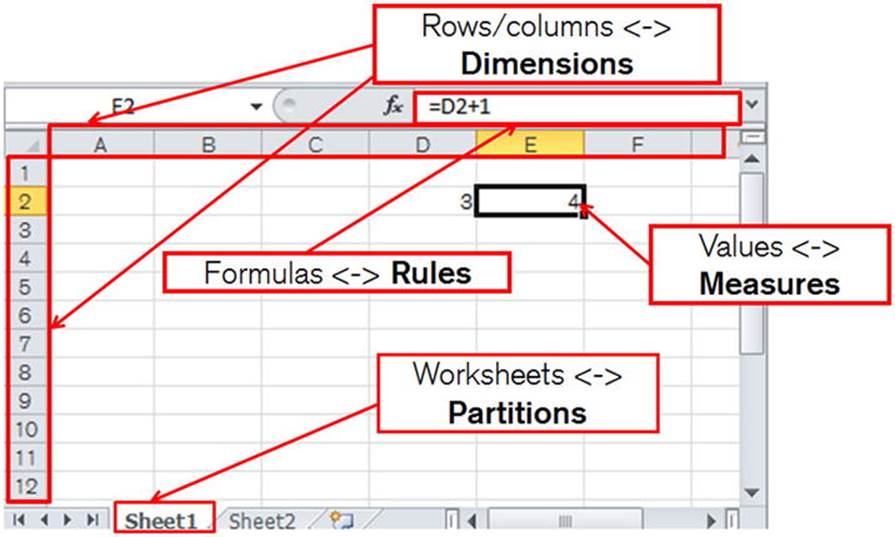
Figure 7-1. Comparing Excel and MODEL clause concepts
· An Excel workbook is split into one or more worksheets. The equivalent MODEL clause concept is the PARTITION. Yet another use of this overloaded term!
· A worksheet contains a number of values. The equivalent MODEL clause concept is the MEASURE.
· Values in a worksheet are referenced by the row number and the column letter. In a MODEL partition the measures are referenced by DIMENSION values.
· Some values in an Excel spreadsheet are evaluated by formulas. The formulas in a MODEL clause are referred to as RULES.
There are some important differences between the Excel and MODEL clause concepts that are summarized in Table 7-1.
Table 7-1. Differences between Excel and MODEL clause concepts
|
Model Term |
Excel Term |
Differences |
|
Partition |
Worksheet |
It is possible for formulas in one Excel worksheet to reference cells in another. It is not possible for partitions in a model clause to reference each other. |
|
Dimension |
Row and column |
In Excel there are always exactly two dimensions. In a model clause there are one or more. |
|
Measure |
A cell value |
In Excel only one value is referenced by the dimensions. The model clause allows one or more measures. |
|
Rules |
Formulas |
Nested cell references are possible with models. |
A Moving Median with the MODEL Clause
Do you remember that we couldn’t use the MEDIAN as an analytic function with a windowing clause because it isn’t supported? Listing 7-22 shows you how to implement a moving median with the MODEL clause.
Listing 7-22. Implementing a moving median with a MODEL clause
ALTER SESSION FORCE PARALLEL QUERY PARALLEL 3;
SELECT transaction_date,channel_id,cust_id,sales_amount,mov_median,mov_med_avg
FROM t1
MODEL
PARTITION BY (cust_id)
DIMENSION BY (ROW_NUMBER () OVER (PARTITION BY cust_id ORDER BY transaction_date) rn)
MEASURES (transaction_date, channel_id, sales_amount, 0 mov_median, 0 mov_med_avg)
RULES
(
mov_median [ANY] =
MEDIAN (sales_amount)[rn BETWEEN CV()-2 AND CV ()],
mov_med_avg [ANY] = ROUND(AVG(mov_median) OVER (ORDER BY rn ROWS 2 PRECEDING))
)
ORDER BY cust_id,transaction_date,mov_median;
ALTER SESSION ENABLE PARALLEL QUERY;
-- Sample output
TRANSACTION_DATE CHANNEL_ID CUST_ID SALES_AMOUNT MOV_MEDIAN MOV_MED_AVG
05-JAN-2014 2 1 25 25 25
10-JAN-2014 3 1 3100 1562.5 794
15-JAN-2014 4 1 225 225 604
20-JAN-2014 1 1 400 400 729
---------------------------------------------------
| Id | Operation | Name |
---------------------------------------------------
| 0 | SELECT STATEMENT | |
| 1 | PX COORDINATOR | |
| 2 | PX SEND QC (ORDER) | :TQ10002 |
| 3 | SORT ORDER BY | |
| 4 | SQL MODEL ORDERED | |
| 5 | PX RECEIVE | |
| 6 | PX SEND RANGE | :TQ10001 |
| 7 | WINDOW SORT | |
| 8 | PX RECEIVE | |
| 9 | PX SEND RANGE | :TQ10000 |
| 10 | PX BLOCK ITERATOR | |
| 11 | TABLE ACCESS FULL | T1 |
| 12 | WINDOW (IN SQL MODEL) SORT| |
---------------------------------------------------
The code in Listing 7-22 begins by forcing parallel query. I only do this so as to demonstrate the parallelization capabilities of the MODEL clause; the dataset is ordinarily too small to warrant parallel query.
The query begins by selecting all rows and columns from T1 and passing the data to the model clause.
· The first sub-clause we see is the optional PARTITION BY clause. This means that the data for each CUST_ID is treated separately—in its own worksheet, if you will.
· The second sub-clause is the DIMENSION BY clause, and the expression here includes an analytic function. The clause defines a new identifier RN that gives the ordering of the rows in our worksheet by transaction date. Normally I would use a factored subquery in a way analogous to Listing 7-20 to make the query easier to read, but here I am just showing what is possible.
· The MEASURES clause identifies what values are addressed by our RN dimension. These include the remaining columns from T1 as well as two new columns. MOV_MEDIAN will be the median for the three most recent transactions and MOV_MED_AVG will be the average (mean) value of MOV_MED from the three most recent transactions. The identifiers are initialized to zero so that the data types of the measures are known.
· The RULES clause then calculates our missing measures.
The first rule uses MEDIAN as an aggregate function, and in the MODEL clause we can explicitly specify the range of measures to be used. The expression in square brackets on the right-hand side is:
rn BETWEEN CV()-2 AND CV ()
The term CV is an abbreviation for CURRENT_VALUE, a function in the model category that is only legal inside a MODEL clause. The CV function is much like a relative cell reference in Excel. So, for example, when the dimension RN has a value of 7 the expression as a whole would be interpreted as rn BETWEEN 5 and 7. Notice that we are applying the aggregate function in the RULES sub-clause after the analytic function in the DIMENSION BY clause. This is legal because the RULES sub-clause operates independently of the rest of the query block.
The second rule is evaluated after the first and so can use the MOV_MEDIAN measure calculated in the first rule as input, just like the results of one formula in Excel can be input to another. I could have calculated the MOV_MED_AVG in the same way as MOV_MEDIAN, but in this case I have the option to use an analytic function and that is what I have chosen to do.
After the measures have been evaluated by the rules, the results are passed back to the select list and the ORDER BY clause. I have included the MOV_MEDIAN in the ORDER BY clause just to show that it is possible to do so and for no other reason.
The execution plan in Listing 7-22 is somewhat lengthy, but that is more to do with the parallelization than the MODEL clause; individual rules within the model clause are not shown in the execution plan. The first thing about the execution plan I want to mention is the difference between operation 7 and operation 12. Operation 7 is used to evaluate the ROW_NUMBER analytic function outside of the MODEL clause and operation 12 is used to evaluate the AVG analytic function inside the MODEL clause, as you might have guessed from the operation name WINDOW (IN SQL MODEL) SORT. There is no visible operation for the MEDIAN aggregate function. The other thing I want to highlight in the execution plan is operation 6. This examines the value of CUST_ID to determine which parallel query slave to send data to; the parallelization of MODEL clause rule evaluation is always based on the expressions in the PARTITION BY sub-clause to prevent the need for any communication between the parallel query slaves.
Why Not Use PL/SQL?
The MODEL clause seems like heresy! SQL is supposed to be a declarative programming language, and here we are writing a series of rules and specifying not only how the calculations are to be performed but in what order. We have imperative programming languages like PL/SQL with equivalent parallelization capabilities for that, don’t we?
The point to realize is that SQL is declarative and has the ability to operate on multiple rows together. PL/SQL and other imperative languages are imperative and single-row based. What the MODEL clause provides us with is imperative syntax capable of operating on multiple rows at a time. Just imagine how difficult it would be to implement a moving median in PL/SQL!
Summary
It is a recurring theme of this book that the more thoroughly you understand things, the easier it is to correctly analyze problems and identify good solutions to those problems. We began this chapter by a look at the syntax of query blocks because without understanding that syntax some aspects of execution plans would be difficult to follow. We then covered functions. A thorough understanding of the main categories of SQL functions is crucial to understanding the increasing number of performance problems that are unrelated to the selection of an index for accessing a table or determining the correct join order. In particular, we saw how the volume of data processed by analytic functions can make them unattractive in some situations. Finally, we introduced the complex topic of the MODEL clause and explained how it can be used to perform analytic calculations on sets of rows when these calculations aren’t easily performed by other means.
This chapter marks the end of our analysis of the SQL language itself. It is time to now to return to the topic of performance analysis. In Chapter 8 we complete our study of execution plans that we began in Chapter 3.