Expert Oracle SQL: Optimization, Deployment, and Statistics (2014)
PART 2. Advanced Concepts
CHAPTER 8. Advanced Execution Plan Concepts
This chapter covers three major topics: the display of execution plans, parallel execution plans, and global hinting.
I have already shown quite a few parts of an execution plan in this book, and in this chapter I will explain most of the remaining parts, most notably the outline hints section. These additional execution plan sections can be displayed with non-default formatting options. The second major topic in the chapter is a discussion of execution plans for statements that run in parallel. There hasn’t been a lot written about how parallel execution plans work, and in particular there is a lot of confusion about how to interpret such execution plans. I want to spend some time clearing all that confusion up. The CBO’s selection of execution plan can be controlled, or at least influenced, by the use of optimizer hints, and there is far more to the topic of hinting than may have been apparent in this book so far. Thus, the third topic in this chapter is global hints. Global hints allow a programmer to influence the CBO’s treatment of blocks other than the one in which the hint appears. This type of hint is useful for hinting query blocks from data dictionary views without altering the view, among other things.
But let me begin this chapter with the first of the three topics: displaying execution plans.
Displaying Additional Execution Plan Sections
In Chapter 3 I explained the default display of execution plans using the functions in the DBMS_XPLAN package, and in Chapter 4 I explained how additional information from the runtime engine can be displayed in the operation table of DBMS_XPLAN output and in theV$SQL_PLAN_STATISTICS_ALL view. But DBMS_XPLAN can display a lot more information about the CBO’s behavior than has been explained so far. If requested to do so by using non-default formatting options, DBMS_XPLAN will display more information in additional sections below the operation table. I will give a brief overview of the formatting options and then explain how to interpret these additional sections.
DBMS_XPLAN Formatting Options
Table 8-1 summarizes the information about the DBMS_XPLAN display options documented in the PL/SQL Packages and Types Reference Manual:
Table 8-1. Format levels and fine-grained control in calls to DBMS_XPLAN packages
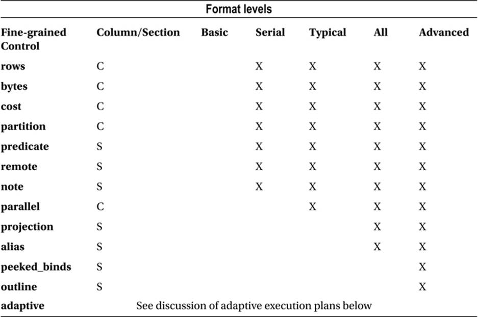
When looking at Table 8-1, bear mind the following points:
· Some optional display data appears in additional columns in the operation table and some appears in additional sections following the operation table. The table shows where each data item appears.
· The BASIC level displays only the Id, Operation, and Name columns of the operation table and, with some obscure exceptions1, no other sections. These basic level columns cannot be suppressed in any display.
· Display levels other than BASIC contain additional columns like Time that cannot be suppressed except by selecting the BASIC level and then adding any desired sections or columns.
· Format keywords are not case sensitive.
· All levels can be customized using fine-grained control together with a minus sign to remove the data or an optional plus sign to add it. So, for example, ‘ADVANCED -COST’ and ‘BASIC +PEEKED_BINDS’ are both legal formats.
· Information about adaptive execution plans is not displayed by any level and must be explicitly added with +ADAPTIVE. Explicitly adding ADAPTIVE to the BASIC level doesn’t work.
· Runtime statistics are displayed using format options as described in Chapter 4. So to obtain the fullest possible display from DBMS_XPLAN.DISPLAY_CURSOR you need to specify ‘ADVANCED ALLSTATS LAST ADAPTIVE’ for the format parameter.
· All levels are documented except ADVANCED and all fine-grained controls are documented except PEEKED_BINDS and OUTLINE.
· The SERIAL level still displays parallel operations for statements executed in parallel. Only the columns in the operation table relating to parallel operations are suppressed.
· Some options don’t apply to all procedures in the DBMS_XPLAN package. For example, PEEKED_BINDS is only valid for DBMS_XPLAN.DISPLAY_CURSOR and PREDICATE information is not displayed in the output of DBMS_XPLAN.DISPLAY_AWR.
I have already explained that if you need detailed information about individual row source operations you had best look at the view V$SQL_PLAN_STATISTICS_ALL, so I will focus on the additional sections of the execution plan, presenting them in the order in which they appear.
Running EXPLAIN PLAN for Analysis
The listings in the remaining sections of this chapter use tables created as in Listing 8-1.
Listing 8-1. Creating tables and a loopback database link for execution plan demonstrations
CREATE PUBLIC DATABASE LINK "loopback"
USING 'localhost:1521/orcl'; -- Customize for your database name and port
CREATE /*+ NO_GATHER_OPTIMIZER_STATISTICS */ TABLE t1 AS
SELECT ROWNUM c1 FROM DUAL CONNECT BY LEVEL <= 100;
CREATE /*+ NO_GATHER_OPTIMIZER_STATISTICS */ TABLE t2 AS
SELECT ROWNUM c2 FROM DUAL CONNECT BY LEVEL <= 100;
CREATE /*+ NO_GATHER_OPTIMIZER_STATISTICS */ TABLE t3 AS
SELECT ROWNUM c3 FROM DUAL CONNECT BY LEVEL <= 100;
CREATE /*+ NO_GATHER_OPTIMIZER_STATISTICS */ TABLE t4 AS
SELECT ROWNUM c4 FROM DUAL CONNECT BY LEVEL <= 100;
Listing 8-1 creates four tables, each with a single column. To test remote access I have also created a loopback database link. The listing assumes that the database is called ORCL and that the SQLNET port is set to the default of 1521. This is a highly insecure approach, and to test the examples you will probably have to change the database link creation statement to meet your needs.
The listings that follow in the next few sections contain both statements and execution plans. Unless otherwise stated the execution plans should be obtained using EXPLAIN PLAN and a call to DBMS_XPLAN.DISPLAY that specifies the BASIC level with the suitable fine-grained control specified in the section in which the listing appears. BASIC level has been used to keep the operation table as uncluttered as possible so that focus is drawn to the other aspects of the execution plan under discussion.
Query Blocks and Object Alias
If the ALIAS fine-grained control is specified or implied then a section detailing the query blocks and objects used in the explained statement appears immediately after the operation table. Listing 8-2 is a simple query that helps demonstrate the meaning of this section.
Listing 8-2. Simple query with three query blocks
WITH q1 AS (SELECT /*+ no_merge */
c1 FROM t1)
,q2 AS (SELECT /*+ no_merge */
c2 FROM t2)
SELECT COUNT (*)
FROM q1, q2 myalias
WHERE c1 = c2;
Plan hash value: 1978226902
-------------------------------------
| Id | Operation | Name |
-------------------------------------
| 0 | SELECT STATEMENT | |
| 1 | SORT AGGREGATE | |
| 2 | HASH JOIN | |
| 3 | VIEW | |
| 4 | TABLE ACCESS FULL| T1 |
| 5 | VIEW | |
| 6 | TABLE ACCESS FULL| T2 |
-------------------------------------
Query Block Name / Object Alias (identified by operation id):
-------------------------------------------------------------
1 - SEL$3
3 - SEL$1 / Q1@SEL$3
4 - SEL$1 / T1@SEL$1
5 - SEL$2 / MYALIAS@SEL$3
6 - SEL$2 / T2@SEL$2
The simple statement in Listing 8-2 could, of course, be made even simpler by eliminating the two factored subqueries and instead just joining T1 and T2. In fact, if the NO_MERGE hints were removed the CBO would apply the simple view merging transformation to do that for us. As it is, the three query blocks aren’t merged and all appear in the final execution plan.
The CBO has provided default names for these three query blocks. These names are SEL$1, SEL$2, and SEL$3 and are allocated in the order in which the SELECT keywords appear in the original statement. The ALIAS section of the execution plan display indicates the query block with which the operations are associated. Where applicable, an object alias is also shown. Because operation 2 is associated with the same query block as operation 1 and there is no object alias to display, operation 2 isn’t shown in the ALIAS section at all; SEL$3 is implied.
For tables T1 and T2 I didn’t specify an alias in the FROM clause so the table name itself is shown for the object alias of operations 4 and 6. You will notice, however, that the table names have been qualified by the name of the query block preceded by an ‘@’ symbol. So for operation 4T1@SEL$1 means the row source named T1 that appears in the FROM clause of SEL$1. This need to qualify row source names arises because the same object (or alias) can be used multiple times in different query blocks within the same SQL statement.
Notice that the alias may be for an object other than a table. Operation 3 references Q1, a factored subquery that was not given an alias in the main clause of Listing 8-2. Operation 5 references MYALIAS, the alias I gave for Q2 in the main query (SEL$3).
Listing 8-3 shows what happens when we remove one of the NO_MERGE hints.
Listing 8-3. Query block merging
WITH q1 AS (SELECT c1 FROM t1)
,q2 AS (SELECT /*+ no_merge */
c2 FROM t2)
SELECT COUNT (*)
FROM q1, q2 myalias
WHERE c1 = c2;
Plan hash value: 3055011902
-------------------------------------
| Id | Operation | Name |
-------------------------------------
| 0 | SELECT STATEMENT | |
| 1 | SORT AGGREGATE | |
| 2 | HASH JOIN | |
| 3 | TABLE ACCESS FULL | T1 |
| 4 | VIEW | |
| 5 | TABLE ACCESS FULL| T2 |
-------------------------------------
Query Block Name / Object Alias (identified by operation id):
-------------------------------------------------------------
1 - SEL$F1D6E378
3 - SEL$F1D6E378 / T1@SEL$1
4 - SEL$2 / MYALIAS@SEL$3
5 - SEL$2 / T2@SEL$2
The operation table now has one less row because the removal of the NO_MERGE hint in the first factored subquery has allowed SEL$1 and SEL$3 to be merged. However, the ALIAS section has suddenly become more difficult to parse. What is that gobbledygook alias for operations 1 and 3? This hexadecimal name is actually a name assigned by the CBO by hashing SEL$1 and SEL$3. It turns out that in all releases up to and including 12cR1 (at least) this apparently random name is always precisely the same when SEL$1 is merged into SEL$3 (but not vice versa) irrespective of the statement, the database instance, or the database version! The only factors that determine the name of the merged query block are the names of the blocks being merged.
Operation 3 demonstrates another interesting point. Notice how the referencing query block (SEL$F1D6E378 left of the slash) is the query block related to the operation, but the referenced query block (SEL$1 on the right of the slash) is the original query block from where the referenced object appears.
When it comes to global hinting we might need to rely on these names, but despite the stability of these names it is actually best practice to explicitly name query blocks when global hints are used. Listing 8-4 shows us how.
Listing 8-4. Naming query blocks using the QB_NAME hint
WITH q1 AS (SELECT /*+ qb_name(qb1)*/
c1 FROM t1)
,q2 AS (SELECT /*+ no_merge */
c2 FROM t2)
SELECT /*+ qb_name(qb2)*/
COUNT (c1)
FROM q1, q2 myalias
WHERE c1 = c2;
Plan hash value: 3055011902
-------------------------------------
| Id | Operation | Name |
-------------------------------------
| 0 | SELECT STATEMENT | |
| 1 | SORT AGGREGATE | |
| 2 | HASH JOIN | |
| 3 | TABLE ACCESS FULL | T1 |
| 4 | VIEW | |
| 5 | TABLE ACCESS FULL| T2 |
-------------------------------------
Query Block Name / Object Alias (identified by operation id):
-------------------------------------------------------------
1 - SEL$86DECE37
3 - SEL$86DECE37 / T1@QB1
4 - SEL$1 / MYALIAS@QB2
5 - SEL$1 / T2@SEL$1
Because we have explicitly renamed SEL$1 to QB1 and SEL$3 to QB2 by means of QB_NAME hints, the fully qualified object aliases have been changed for operations 3 and 4 in Listing 8-4. Furthermore, the query block name for operation 5 has changed from SEL$2 to SEL$1, as operation 5 is now associated with the first unnamed query block in the statement. What is more, the gobbledygook name for the merged query block has changed; whenever a query block named QB1 is merged into QB2 the resulting query block is named SEL$86DECE37. Listing 8-5shows query block naming in a DML statement.
Listing 8-5. Additional query block with multi-table insert
INSERT ALL
INTO t1 (c1)
WITH q1 AS (SELECT /*+ qb_name(qb1) */
c1 FROM t1)
,q2 AS (SELECT /*+ no_merge */
c2 FROM t2)
SELECT /*+ qb_name(qb2) */
COUNT (c1)
FROM q1, q2 myalias
WHERE c1 = c2;
Plan hash value: 3420834736
---------------------------------------
| Id | Operation | Name |
---------------------------------------
| 0 | INSERT STATEMENT | |
| 1 | MULTI-TABLE INSERT | |
| 2 | VIEW | |
| 3 | SORT AGGREGATE | |
| 4 | HASH JOIN | |
| 5 | TABLE ACCESS FULL | T1 |
| 6 | VIEW | |
| 7 | TABLE ACCESS FULL| T2 |
| 8 | INTO | T1 |
---------------------------------------
Query Block Name / Object Alias(identified by operation id):
-------------------------------------------------------------
1 - SEL$1
2 - SEL$86DECE37 / from$_subquery$_002@SEL$1
3 - SEL$86DECE37
5 - SEL$86DECE37 / T1@QB1
6 - SEL$2 / MYALIAS@QB2
7 - SEL$2 / T2@SEL$2
The presence of the keyword ALL following the INSERT keyword in Listing 8-5 makes it syntactically a multi-table operation even though we are only inserting data into T1. However, the query block associated with the unmerged selection from T2 (operation 7 in Listing 8-5) has changed from SEL$1 to SEL$2. What has happened here is that a hidden query block has been added. The name of our merged query block hasn’t changed though, because it is still formed by merging QB1 into QB2. When we look at global hinting later in this chapter the significance of this will become clearer.
In real life, the statements we are asked to tune are usually far more complicated than the simple examples that I have given so far. Listing 8-6 is a little more realistic.
Listing 8-6. Multiple query-block types
ALTER SESSION SET star_transformation_enabled=temp_disable;
INSERT /*+ APPEND */ INTO t2 (c2)
WITH q1
AS (SELECT *
FROM book.t1@loopback t1)
SELECT
COUNT (*)
FROM (SELECT *
FROM q1, t2
WHERE q1.c1 = t2.c2
UNION ALL
SELECT *
FROM t3, t4
WHERE t3.c3 = t4.c4
-- ORDER BY 1 ... see the explanation of column projections below
)
,t3
WHERE c1 = c3;
COMMIT;
ALTER SESSION SET star_transformation_enabled=false;
Plan hash value: 2044158967
-------------------------------------------------
| Id | Operation | Name |
-------------------------------------------------
| 0 | INSERT STATEMENT | |
| 1 | LOAD AS SELECT | T2 |
| 2 | OPTIMIZER STATISTICS GATHERING | |
| 3 | SORT AGGREGATE | |
|* 4 | HASH JOIN | |
| 5 | TABLE ACCESS FULL | T3 |
| 6 | VIEW | |
| 7 | UNION-ALL | |
|* 8 | HASH JOIN | |
| 9 | REMOTE | T1 |
| 10 | TABLE ACCESS FULL | T2 |
|* 11 | HASH JOIN | |
| 12 | TABLE ACCESS FULL | T3 |
| 13 | TABLE ACCESS FULL | T4 |
-------------------------------------------------
Query Block Name / Object Alias (identified by operationid):
-------------------------------------------------------------
1 - SEL$2
5 - SEL$2 / T3@SEL$2
6 - SET$1 / from$_subquery$_003@SEL$2
7 - SET$1
8 - SEL$F1D6E378
9 - SEL$F1D6E378 / T1@SEL$1
10 - SEL$F1D6E378 / T2@SEL$3
11 - SEL$4
12 - SEL$4 / T3@SEL$4
13 - SEL$4 / T4@SEL$4
![]() Caution because of the unpredictable behaviour of dynamic sampling, the operations on lines 9 and 10 may be transposed.
Caution because of the unpredictable behaviour of dynamic sampling, the operations on lines 9 and 10 may be transposed.
Listing 8-6 shows a single-table INSERT statement that includes four occurrences of the SELECT keyword. As a single-table INSERT statement doesn’t introduce an extra query block in the same way that a multi-table INSERT does, these four query blocks have been named SEL$1,SEL$2, SEL$3, and SEL$4. However, SEL$3 and SEL$4 are operands of a UNION ALL operator, and, as I explained at the beginning of Chapter 7, this results in the creation of a new query block that has been named SET$1.SET$1 is an inline view referenced in the main query (SEL$2). Unlike real tables, data dictionary views, and factored subqueries, there is no default object alias for an inline view. And since an alias isn’t explicitly specified for the inline view in Listing 8-6, the CBO has made up the name from$_subquery$_003@SEL$2 and shown it for operation 6.
I would like to conclude this explanation of the ALIAS section of an execution plan with two observations:
· Listing 8-6 merges SEL$1 into SEL$3; the resulting query block name, SEL$F1D6E378, is the same as that in Listing 8-3. In both cases the name is formed by hashing SEL$1 and SEL$3.
· There is no entry for operations 2, 3, and 4 in Listing 8-6 because there is no object alias; the associated query block is the same as operation 1, i.e., SEL$2.
Outline Data
Following the ALIAS section of an execution plan display is the OUTLINE section. To explain the purpose and use of this OUTLINE section I will use the same statement as that provided in Listing 8-6. Listing 8-7 just shows the OUTLINE section.
Listing 8-7. Outline data for INSERT in Listing 8-6
01 /*+
02 BEGIN_OUTLINE_DATA
03 USE_HASH(@"SEL$F1D6E378" "T1"@"SEL$1")
04 LEADING(@"SEL$F1D6E378" "T1"@"SEL$1" "T2"@"SEL$3")
05 FULL(@"SEL$F1D6E378" "T1"@"SEL$1")
06 FULL(@"SEL$F1D6E378" "T2"@"SEL$3")
07 USE_HASH(@"SEL$4" "T4"@"SEL$4")
08 LEADING(@"SEL$4" "T3"@"SEL$4" "T4"@"SEL$4")
09 FULL(@"SEL$4" "T4"@"SEL$4")
10 FULL(@"SEL$4" "T3"@"SEL$4")
11 USE_HASH(@"SEL$2" "from$_subquery$_003"@"SEL$2")
12 LEADING(@"SEL$2" "T3"@"SEL$2" "from$_subquery$_003"@"SEL$2")
13 NO_ACCESS(@"SEL$2" "from$_subquery$_003"@"SEL$2")
14 FULL(@"SEL$2" "T3"@"SEL$2")
15 FULL(@"INS$1" "T2"@"INS$1")
16 OUTLINE(@"SEL$1")
17 OUTLINE(@"SEL$3")
18 OUTLINE_LEAF(@"INS$1")
19 OUTLINE_LEAF(@"SEL$2")
20 OUTLINE_LEAF(@"SET$1")
21 OUTLINE_LEAF(@"SEL$4")
22 MERGE(@"SEL$1")
23 OUTLINE_LEAF(@"SEL$F1D6E378")
24 ALL_ROWS
25 OPT_PARAM('star_transformation_enabled' 'temp_disable')
26 DB_VERSION('12.1.0.1')
27 OPTIMIZER_FEATURES_ENABLE('12.1.0.1')
28 IGNORE_OPTIM_EMBEDDED_HINTS
29 END_OUTLINE_DATA
30 */
This section of an execution plan is just full of that hexadecimal gobbledygook! Hopefully the explanation in the previous section of how query blocks and object aliases are named makes it a little less difficult to parse, but the section is clearly not designed for human readability. Be aware that the line numbers in Listing 8-7 will not appear in real life. I have added line numbers to assist with the explanations that follow.
![]() Note DML statements make use of additional “query blocks“ that don’t appear in the alias section. You will see that operation 15 makes reference to a query blocked named INS$1.DELETE, MERGE, and UPDATE statements include a DEL$1, MRG$1, and UPD$1 “query block” respectively. If you explain a CREATE INDEX or ALTER INDEX statement you will also see mention of a CRI$1 “query block.”
Note DML statements make use of additional “query blocks“ that don’t appear in the alias section. You will see that operation 15 makes reference to a query blocked named INS$1.DELETE, MERGE, and UPDATE statements include a DEL$1, MRG$1, and UPD$1 “query block” respectively. If you explain a CREATE INDEX or ALTER INDEX statement you will also see mention of a CRI$1 “query block.”
The purpose of the OUTLINE section of an execution plan is to provide all the hints necessary to fully specify the execution plan for the statement. If you just take the section, which conveniently includes the /*+ */ hint syntax, and paste it into your statement at any point where a hint is legal, the theory is that while the execution plan remains legal it will not change regardless of any changes to object statistics, system statistics, or most initialization parameters; you will have removed all flexibility from the CBO.
These types of hints are actually what are kept in stored outlines and SQL plan baselines, but in fact they do not fully specify the execution plan for Listing 8-6. Let us take a detailed look at the different types of hints so as to understand what is missing.
Outline Interpretation Hints
When customers of Oracle upgraded from 9i to 10g many found that their stored outlines no longer worked as expected. The problem was that the interpretation of hints changed. These days hints like those on lines 24, 25, 26, and 27 of Listing 8-7 control the precise way that the remaining hints are interpreted. Of course, the ALL_ROWS hint might be replaced by one of the FIRST_ROWS variants if you have specified such a hint in your code or have a non-default setting of the OPTMIZER_MODE initialization parameter. The value of the parameter passed toOPTIMIZER_FEATURES_ENABLE may also differ because of the database version or because of a hint or initialization parameter setting.
How these parameters work together with the undocumented DB_VERSION hint need not concern us. All we need to know is that the intention is to avoid changes in behavior when the database version or initialization parameters change. If there are any non-default settings for optimizer initialization parameters, such as the STAR_TRANSFORMATION_ENABLED setting that I changed before explaining the query, one or more OPT_PARAM hints will also be present, such as that found on line 25.
Identifying Outline Data
The hints on lines 2, 28, and 29 in Listing 8-7 work together to ensure that the outline hints are treated differently from other hints in the statement. The IGNORE_OPTIM_EMBEDDED_HINTS hint tells the CBO to ignore most hints in the SQL statement except those that are bracketed byBEGIN_OUTLINE_DATA and END_OUTLINE_DATA hints. I have emphasized the word most because there are a number of hints that aren’t implemented in the OUTLINE section of an execution plan, and thankfully these aren’t ignored.
THE TERM “OUTLINE”
The term “outline” is somewhat overloaded, and to avoid confusion I need to explain its different uses:
· There is a section in the output of DBMS_XPLAN functions generated as a result of the OUTLINE fine-grained control that has the heading Outline Data.
· The content of the outline section includes hints that are individually referred to as outline hints, and the entire set is referred to simply as an outline. These outline hints are bracketed by the two hints BEGIN_OUTLINE_DATA and END_OUTLINE_DATA.
· Outline hints are the basis for the implementation of plan stability features such as stored outlines and SQL plan baselines.
· Outline hints can be pasted into SQL statements where they continue to be referred to as outline hints. Hints other than those bracketed by the BEGIN_OUTLINE_DATA and END_OUTLINE_DATA hints are referred to as embedded hints.
· And if that isn’t confusing enough, one of these outline hints is named OUTLINE and another is named OUTLINE_LEAF.
Hopefully this helps a bit.
An example of an embedded hint that isn’t ignored by IGNORE_OPTIM_EMBEDDED_HINTS is APPEND. APPEND causes a serial direct-path load to occur. Neither the APPEND hint in Listing 8-6, nor any alternative hint that performs the same function, makes an appearance inListing 8-7, but a serial direct-path load has still occurred. To make this point clearer Listing 8-8 shows how we might move our outline hints into Listing 8-6 to prevent changes to the execution plan.
Listing 8-8. Use of outline hints in source code
INSERT /*+ APPEND */
INTO t2 (c2)
WITH q1
AS (SELECT *
FROM book.t1@loopback t1)
SELECT /*+
BEGIN_OUTLINE_DATA
<other hints suppressed for brevity>
IGNORE_OPTIM_EMBEDDED_HINTS
END_OUTLINE_DATA
*/
COUNT (*)
FROM (SELECT *
FROM q1, t2
WHERE q1.c1 = t2.c2
UNION ALL
SELECT *
FROM t3, t4
WHERE t3.c3 = t4.c4)
,t3
WHERE c1 = c3;
The highlighted hints in Listing 8-8 originated from Listing 8-7 but have been shortened for brevity. If you look at the execution plan for Listing 8-8 you will see that it is unchanged from that of Listing 8-6 and in particular that operation 1 is still LOAD AS SELECT. If the APPEND hint is removed from Listing 8-8 then operation 1 becomes LOAD TABLE CONVENTIONAL, as no instruction to use direct-path load appears in the outline hints.
![]() Note Non-default values for optimizer parameters, such as _optimizer_gather_stats_on_load, will also be ignored unless there is an appropriate OPT_PARAM hint included in the outline hints. This is because of the presence of the OPTIMIZER_FEATURES_ENABLE hint that resets optimizer parameters to the default for that release.
Note Non-default values for optimizer parameters, such as _optimizer_gather_stats_on_load, will also be ignored unless there is an appropriate OPT_PARAM hint included in the outline hints. This is because of the presence of the OPTIMIZER_FEATURES_ENABLE hint that resets optimizer parameters to the default for that release.
For a complete list of hints that are not implemented in an outline you can look at the view V$SQL_HINT. All rows where OUTLINE_VERSION is NULL identify hints that, if included in source code, will not be implemented in an outline and will not be ignored byIGNORE_OPTIM_EMBEDDED_HINTS. Hints that are excluded from outlines include RESULT_CACHE, which we discussed in Chapter 4, as well as MATERIALIZE and INLINE, which control the behavior of factored subqueries. We will look at the materialization of factored subqueries in Chapter 13.
![]() Note An amusing paradox arises when IGNORE_OPTIM_EMBEDDED_HINTS is supplied as an embedded hint outside of an outline. In fact, such a hint has no effect. This in effect means that it ignored itself!
Note An amusing paradox arises when IGNORE_OPTIM_EMBEDDED_HINTS is supplied as an embedded hint outside of an outline. In fact, such a hint has no effect. This in effect means that it ignored itself!
I am emphasizing the distinction between hints that appear in outlines and those that don’t because many people remove all other embedded hints from their SQL statement when they paste outline hints into their code. Don’t remove any embedded hints until you are sure that they are truly unnecessary!
Final Query Block Structure
The hints OUTLINE_LEAF and OUTLINE appear in Listing 8-7 on lines 16, 17, 18, 19, 20, 21, and 23. These hints indicate which query blocks exist in the final execution plan (OUTLINE_LEAF) and which were merged or otherwise transformed out of existence (OUTLINE).2
It is about time I gave you a warning about the undocumented hints you see in outlines. You shouldn’t try changing them or using them outside of outlines unless you know what you are doing. For example, if you want to suppress view merging you could use OUTLINE_LEAF to do so. However, it is much safer to use the documented NO_MERGE hint for this purpose in the way I have done several times in this chapter. Reserve the use of hints like OUTLINE and OUTLINE_LEAF to the occasions when you paste outline hints unaltered into your code.
Query Transformation Hints
The MERGE hint on line 22 in Listing 8-7 shows the use of the simple view-merging query transformation applied to query block SEL$1. We will cover most of the query transformations available to the CBO in Chapter 13, and all discretionary query transformations that are used in a statement will be reflected in an outline by hints such as MERGE.
Comments
The NO_ACCESS hint on line 13 in Listing 8-7 is a bit of a mystery to me. It documents the fact that the CBO did not merge a query block. It doesn’t actually have any effect when you place it in your code, and it doesn’t seem to matter if you remove it from the outline. It seems to be just a comment.
Final State Optimization Hints
This hints on lines 3 to 12 and on lines 14 and 15 in Listing 8-7 look almost like the normal embedded hints that appear in SQL statements. They control join order, join method, and access method. I say almost because they include global hint syntax and fully qualified object aliases, which, although legal, are rarely found in the source code of SQL statements. We will look into global hints in more detail later in the chapter.
We have now categorized all of the outline hints in Listing 8-7. Let us move on to other sections of the DBMS_XPLAN output.
Peeked Binds
When a call is made to DBMS_XPLAN.DISPLAY_CURSOR, the PEEKED_BINDS section follows the OUTLINE section. Listing 8-6 cannot be used to demonstrate PEEKED_BINDS for two reasons:
· The statement doesn’t have any bind variables.
· The statement uses a database link and because of this, in releases prior to 12cR1, no bind variable peeking is performed.
So for the purposes of the PEEKED_BINDS section I will use the script shown in Listing 8-9.
Listing 8-9. Local database query demonstrating peeked binds
DECLARE
dummy NUMBER := 0;
BEGIN
FOR r IN (WITH q1 AS (SELECT /*+ TAG1*/
* FROM t1)
SELECT *
FROM (SELECT *
FROM q1, t2
WHERE q1.c1 = t2.c2 AND c1 > dummy
UNION ALL
SELECT *
FROM t3, t4
WHERE t3.c3 = t4.c4 AND c3 > dummy)
,t3
WHERE c1 = c3)
LOOP
NULL;
END LOOP;
END;
/
SET LINES 200 PAGES 0
SELECT p.*
FROM v$sql s
,TABLE (
DBMS_XPLAN.display_cursor (s.sql_id
,s.child_number
,'BASIC +PEEKED_BINDS')) p
WHERE sql_text LIKE 'WITH%SELECT /*+ TAG1*/%';
EXPLAINED SQL STATEMENT:
------------------------
WITH Q1 AS (SELECT /*+ TAG1 */ * FROM T1) SELECT * FROM (SELECT * FROM
Q1, T2 WHERE Q1.C1 = T2.C2 AND C1 > :B1 UNION ALL SELECT * FROM T3, T4
WHERE T3.C3 = T4.C4 AND C3 > :B1 ) ,T3 WHERE C1 = C3
Plan hash value: 2648033210
--------------------------------------
| Id | Operation | Name |
--------------------------------------
| 0 | SELECT STATEMENT | |
| 1 | HASH JOIN | |
| 2 | TABLE ACCESS FULL | T3 |
| 3 | VIEW | |
| 4 | UNION-ALL | |
| 5 | HASH JOIN | |
| 6 | TABLE ACCESS FULL| T1 |
| 7 | TABLE ACCESS FULL| T2 |
| 8 | HASH JOIN | |
| 9 | TABLE ACCESS FULL| T3 |
| 10 | TABLE ACCESS FULL| T4 |
--------------------------------------
Peeked Binds (identified by position):
--------------------------------------
1 - :B1 (NUMBER): 0
2 - :B1 (NUMBER, Primary=1)
Unlike the earlier examples in this chapter that imply a call to EXPLAIN PLAN followed by a call to DBMS_XPLAN.DISPLAY, Listing 8-9 actually runs a statement and then calls DBMS_XPLAN.DISPLAY_CURSOR to produce the output. You will see that I included the string TAG1in the comment of the statement. This comment appears to the PL/SQL compiler as a hint (it isn’t, of course) and so the comment isn’t removed. After running the statement and discarding the rows returned, I call DBMS_XPLAN.DISPLAY_CURSOR using a left lateral join with V$SQL to identify the SQL_ID. I will cover left lateral joins when we talk about join methods in Chapter 11. The output of the call to DBMS_XPLAN.DISPLAY_CURSOR is also shown in Listing 8-9.
We can see that when the query was parsed the value of the bind variable :B1 was looked at in case its value might influence the choice of execution plan. The bind variable was added by PL/SQL as a result of the use of the PL/SQL variable I have named DUMMY.DUMMY was used twice, but there is no need to peek at its value twice. That is the meaning of the Primary=1 part of the output—it indicates that the value of the second use of the bind variable is taken from the first.
It is worthwhile repeating that bind variables are only peeked at when the statement is parsed. With a few exceptions, such as adaptive cursor sharing, the second and subsequent executions of a statement with different values for the bind variables will not cause any more peeking, and the output from DBMS_XPLAN.DISPLAY_CURSOR will not be updated by such calls.
Predicate Information
The PREDICATE section of the DBMS_XPLAN function calls appears after any PEEKED_BINDS section. We have already covered filter predicates in Chapter 3 because the default output level of the DBMS_XPLAN functions is TYPICAL and the PREDICATE section is included in theTYPICAL level. For completeness, Listing 8-10 shows the filter predicates of the statement in Listing 8-6.
Listing 8-10. Predicate information for query in Listing 8-6
Predicate Information (identified by operation id):
---------------------------------------------------
4 - access("C1"="C3")
8 - access("T1"."C1"="T2"."C2")
11 - access("T3"."C3"="T4"."C4")
The access predicates in this case relate to the three HASH JOIN operations.
Column Projection
The next section of the DBMS_XPLAN output to be displayed shows the columns that are returned by the various row source operations. These may not be the same as those specified by the programmer because in some cases the CBO can determine that they are not required and then eliminate them. Listing 8-11 shows the column projection data for the statement in Listing 8-6.
Listing 8-11. Column projection information for the query in Listing 8-6
Column Projection Information (identified by operation id):
-----------------------------------------------------------
1 - SYSDEF[4], SYSDEF[16336], SYSDEF[1], SYSDEF[112], SYSDEF[16336]
2 - (#keys=3) COUNT(*)[22]
3 - (#keys=0) COUNT(*)[22]
4 - (#keys=1) "C3"[NUMBER,22], "C1"[NUMBER,22]
5 - (rowset=200) "C3"[NUMBER,22]
6 - "C1"[NUMBER,22]
7 - STRDEF[22]
8 - (#keys=1) "T1"."C1"[NUMBER,22], "T2"."C2"[NUMBER,22]
9 - "T1"."C1"[NUMBER,22]
10 - (rowset=200) "T2"."C2"[NUMBER,22]
11 - (#keys=1) "T3"."C3"[NUMBER,22], "T4"."C4"[NUMBER,22]
12 - (rowset=200) "T3"."C3"[NUMBER,22]
13 - (rowset=200) "T4"."C4"[NUMBER,22]
This section can be useful when you are assessing memory requirements, as you can see not only the names of the columns but also the data types and the size of the columns. Operations 4, 8, and 11 include the text (#keys=1). This means that there is one column used in the join. The columns used in a join or sort are always listed first so, for instance, operation 11 uses T3.C3 for the hash join.
I find the output associated with operation 3 to be amusing. The text (#keys=0) indicates that no columns were used in the sort. As I explained in Chapter 3, there isn’t a sort with SORT AGGREGATE! You will also see that operation 7, the UNION-ALL operator, shows an identifier name as STRDEF. I have no idea what STRDEF stands for, but it is used for internally generated column names.
![]() Note The ORDER BY clause in a set query block must specify positions or aliases rather than explicit expressions. A commented-out line in bold in Listing 8-6 gives an example.
Note The ORDER BY clause in a set query block must specify positions or aliases rather than explicit expressions. A commented-out line in bold in Listing 8-6 gives an example.
Remote SQL
Because Listing 8-6 uses a database link, a portion of the statement needs to be sent to the far side of the link for processing. Listing 8-12 shows this SQL.
Listing 8-12. Remote SQL information for query in Listing 8-6
Remote SQL Information (identified by operation id):
----------------------------------------------------
9 - SELECT /*+ */ "C1" FROM "BOOK"."T1" "T1" (accessing 'LOOPBACK' )
You will see that the text of the query sent to the "remote" database has been altered to quote identifiers, specify the schema (in my case BOOK), and add an object alias. If hints were supplied in the original statement then the appropriate subset would be included in the query sent to the "remote" database. This remote SQL statement will, of course, have its own execution plan, but if you need to examine this you will have to do so separately on the remote database.
Adaptive Plans
Adaptive execution plans are new to 12cR1 and are probably the most well-known of the new adaptive features of that release. With the exception of a note, information about execution plan adaptation is only shown when ADAPTIVE is explicitly added to the format parameter of theDBMS_XPLAN call. Contrary to the documentation, ADAPTIVE is a fine-grained control, not a format level.
The idea is of adaptive plans is as follows: You have two possible plans. You start with one and if that doesn’t work out you switch to the other in mid-flight. Although hybrid parallel query distribution, which we will discuss in the context of parallel queries later in this chapter, is very similar, as of 12.1.0.1 the only truly adaptive mechanism is the table join.
The adaptive join works like this. You find some matching rows from one of the tables being joined and see how many you get. If you get a small number you can access the second table being joined with a nested loops join. If it seems like you are getting a lot then at some point you will give up on the nested loops and start working on a hash join.
We will discuss the ins and outs of nested loops joins and hash joins in Chapter 11, but right now all we need to focus on is understanding what the execution plans are trying to tell us.
Not all joins are adaptive. In fact most are not, so for my demonstration I have had to rely on the example provided in the SQL Tuning Guide. Listing 8-13 shows my adaptation of the SQL Tuning Guide’s example of adaptive joins.
Listing 8-13. Use of adaptive execution plans
ALTER SYSTEM FLUSH SHARED_POOL;
SET LINES 200 PAGES 0
VARIABLE b1 NUMBER;
EXEC :b1 := 15;
SELECT product_name
FROM oe.order_items o, oe.product_information p
WHERE unit_price = :b1 AND o.quantity > 1 AND p.product_id = o.product_id;
SELECT *
FROM TABLE (DBMS_XPLAN.display_cursor (format => 'TYPICAL +ADAPTIVE'));
EXEC :b1 := 1000;
SELECT product_name
FROM oe.order_items o, oe.product_information p
WHERE unit_price = :b1 AND o.quantity > 1 AND p.product_id = o.product_id;
SELECT *
FROM TABLE (DBMS_XPLAN.display_cursor (format => 'TYPICAL'));
EXEC :b1 := 15;
SELECT product_name
FROM oe.order_items o, oe.product_information p
WHERE unit_price = :b1 AND o.quantity > 1 AND p.product_id = o.product_id;
SELECT *
FROM TABLE (DBMS_XPLAN.display_cursor (format => 'TYPICAL'));
Before looking at the output from the code in Listing 8-13, let us look at what it does. Listing 8-13 starts by flushing the shared pool to get rid of any previous runs and then sets up a SQL*Plus variable B1, which is initialized to 15 and used as a bind variable in the query based on the OEexample schema. After the query returns, the execution plan is displayed using DBMS_XPLAN.DISPLAY_CURSOR. Listing 8-13 specifies ADAPTIVE in the call to DBMS_XPLAN.DISPLAY_CURSOR to show the bits of the execution plan we are interested in.
The value of the SQL*Plus variable B1 is then changed from 15 to 1000 and the query is run a second time. Finally, B1 is changed back to 15 and the query is rerun for the third and final time. After the second and third runs of our query we don’t list the adaptive parts of the execution plan in our call to DBMS_XPLAN.DISPLAY_CURSOR.
Listing 8-14 shows the output from Listing 18-13.
Listing 8-14. Execution plans from an adaptive query run multiple times
System altered.
PL/SQL procedure successfully completed.
Screws <B.28.S>
<cut>
Screws <B.28.S>
13 rows selected.
SQL_ID g4hyzd4v4ggm7, child number 0
-------------------------------------
SELECT product_name FROM oe.order_items o, oe.product_information p
WHERE unit_price = :b1 AND o.quantity > 1 AND p.product_id =
o.product_id
Plan hash value: 1553478007
-------------------------------------------------------------------------------------
| Id | Operation | Name | Rows | Time |
-------------------------------------------------------------------------------------
| 0 | SELECT STATEMENT | | | |
| * 1 | HASH JOIN | | 4 | 00:00:01 |
|- 2 | NESTED LOOPS | | | |
|- 3 | NESTED LOOPS | | 4 | 00:00:01 |
|- 4 | STATISTICS COLLECTOR | | | |
| * 5 | TABLE ACCESS FULL | ORDER_ITEMS | 4 | 00:00:01 |
|- * 6 | INDEX UNIQUE SCAN | PRODUCT_INFORMATION_PK | 1 | |
|- 7 | TABLE ACCESS BY INDEX ROWID| PRODUCT_INFORMATION | 1 | 00:00:01 |
| 8 | TABLE ACCESS FULL | PRODUCT_INFORMATION | 1 | 00:00:01 |
-------------------------------------------------------------------------------------
Predicate Information(identified by operation id):
---------------------------------------------------
1 - access("P"."PRODUCT_ID"="O"."PRODUCT_ID")
5 - filter(("UNIT_PRICE"=:B1 AND "O"."QUANTITY">1))
6 - access("P"."PRODUCT_ID"="O"."PRODUCT_ID")
Note
-----
- this is an adaptive plan (rows marked '-' are inactive)
33 rows selected.
PL/SQL procedure successfullycompleted.
no rows selected.
SQL_ID g4hyzd4v4ggm7, child number 1
-------------------------------------
SELECT product_name FROM oe.order_items o, oe.product_information p
WHERE unit_price = :b1 AND o.quantity > 1 AND p.product_id =
o.product_id
Plan hash value: 1255158658
----------------------------------------------------------------------------------
| Id | Operation | Name | Rows | Time |
----------------------------------------------------------------------------------
| 0 | SELECT STATEMENT | | | |
| 1 | NESTED LOOPS | | | |
| 2 | NESTED LOOPS | | 13 | 00:00:01 |
|* 3 | TABLE ACCESS FULL | ORDER_ITEMS | 4 | 00:00:01 |
|* 4 | INDEX UNIQUE SCAN | PRODUCT_INFORMATION_PK | 1 | |
| 5 | TABLE ACCESS BY INDEX ROWID| PRODUCT_INFORMATION | 4 | 00:00:01 |
----------------------------------------------------------------------------------
Predicate Information (identified by operation id):
---------------------------------------------------
3 - filter(("UNIT_PRICE"=:B1AND "O"."QUANTITY">1))
4 - access("P"."PRODUCT_ID"="O"."PRODUCT_ID")
Note
-----
- statistics feedback used for this statement
- this is an adaptive plan
30 rows selected.
PL/SQL procedure successfully completed.
Screws <B.28.S>
<cut>
Screws <B.28.S>
13 rows selected.
SQL_ID g4hyzd4v4ggm7, child number 1
-------------------------------------
SELECT product_name FROM oe.order_items o, oe.product_information p
WHERE unit_price = :b1 AND o.quantity > 1 AND p.product_id =
o.product_id
Plan hash value: 1255158658
----------------------------------------------------------------------------------
| Id | Operation | Name | Rows | Time |
----------------------------------------------------------------------------------
| 0 | SELECT STATEMENT | | | |
| 1 | NESTED LOOPS | | | |
| 2 | NESTED LOOPS | | 13 | 00:00:01 |
|* 3 | TABLE ACCESS FULL | ORDER_ITEMS | 4 | 00:00:01 |
|* 4 | INDEX UNIQUE SCAN | PRODUCT_INFORMATION_PK | 1 | |
| 5 | TABLE ACCESS BY INDEX ROWID| PRODUCT_INFORMATION | 4 | 00:00:01 |
----------------------------------------------------------------------------------
Predicate Information(identified by operation id):
---------------------------------------------------
3 - filter(("UNIT_PRICE"=:B1 AND "O"."QUANTITY">1))
4 - access("P"."PRODUCT_ID"="O"."PRODUCT_ID")
Note
-----
- statistics feedback used for this statement
- this is an adaptive plan
30 rows selected.
The first query returns 13 rows—more than the CBO’s estimate of 4—and by taking a careful look at the first child cursor for this statement (child 0) you can see that a hash join has been used. You can see this by mentally removing the lines with a minus sign that show the alternative plan that was discarded. When we rerun the same SQL statement, this time with a bind variable that results in no rows being returned, we see that a new child cursor has been created (child 1) and that we have used a nested loops join. This time I didn’t use the ADAPTIVE keyword in the format parameter of DBMS_XPLAN.DISPLAY_CURSOR, and the unused portions of the execution plan have not been shown.
![]() Note My thanks to Randolf Geist, who, after several attempts, convinced me that the extra child cursor is actually a manifestation of statistics feedback and not of adaptive plans.
Note My thanks to Randolf Geist, who, after several attempts, convinced me that the extra child cursor is actually a manifestation of statistics feedback and not of adaptive plans.
All this is very impressive, but what happens when we run the query for the third time, using the original value of the bind variable? Unfortunately, we continue to use the nested loops join and don’t revert back to the hash join!
We have already seen one big feature of Oracle database that adapts once and doesn’t adapt again: bind variable peeking. Bind variable peeking didn’t work out well, but hopefully this same shortcoming of adaptive execution plans will be fixed sometime soon.
Result Cache Information
In Chapter 4 I showed how the runtime engine can make use of the result cache. If the result cache is used in a statement, then a section is placed in the output of all DBMS_XPLAN functions that shows its use. This section cannot be suppressed, but it only contains meaningful information when used with DBMS_XPLAN.DISPLAY and even then only when the level is TYPICAL, ALL, or ADVANCED. Listing 8-15 shows a simple example.
Listing 8-15. Result cache information from a simple statement
SET PAGES 0 LINES 300
EXPLAIN PLAN FOR SELECT /*+ RESULT_CACHE */ * FROM DUAL;
Explain complete.
SELECT * FROM TABLE (DBMS_XPLAN.display (format => 'TYPICAL'));
Plan hash value: 272002086
------------------------------------------------------------------------------------------------
| Id | Operation | Name | Rows | Bytes | Cost (%CPU)| Time |
------------------------------------------------------------------------------------------------
| 0 | SELECT STATEMENT | | 1 | 2 | 2 (0)| 00:00:01 |
| 1 | RESULT CACHE | 9p1ghjb9czx4w7vqtuxk5zudg6| | | | |
| 2 | TABLE ACCESS FULL| DUAL | 1 | 2 | 2 (0)| 00:00:01 |
-------------------------------------------------------------------------------------------------
Result Cache Information (identified by operation id):
------------------------------------------------------
1 - column-count=1; attributes=(single-row); name="SELECT /*+ RESULT_CACHE */ * FROM DUAL"
14 rows selected.
Notes
The NOTE section of the execution plan provides textual information that may be useful. There are lots of different types of notes that can appear in this section. We have already seen notes relating to adaptive plans. Here are some more of the notes that I have seen:
- rule based optimizer used (consider using cbo)
- cbqt star transformation used for this statement
- Warning: basic plan statistics not available. These are only collected when:
* hint 'gather_plan_statistics' is used for the statement or
* parameter 'statistics_level' is set to 'ALL', at session or system level
The first note will be displayed when the execution plan is produced by the RBO and not the CBO, perhaps because a RULE hint is used. The second hint is displayed when cost-based query transformation (CBQT) results in a star transformation. The third note is displayed when you have selected a format parameter such as ALLSTATS but the statistics from the runtime engine are not available, perhaps for the reasons given in the note or perhaps because you have used DBMS_XPLAN.DISPLAY and the SQL statement hasn’t actually been run.
In the case of the statement in Listing 8-6 a fourth type of note appears, and this is shown in Listing 8-16.
Listing 8-16. Note for the query in Listing 8-6
Note
-----
- dynamic sampling used for this statement (level=2)
This note is displayed because I used hints to suppress the gathering of statistics on the example tables as they were created. As a consequence, the CBO sampled the data in the tables to generate statistics for its plan evaluation.
That concludes our discussion of execution plan displays. Let us move on to the second major topic of this chapter, parallel execution plans.
Understanding Parallel Execution Plans
When a SQL statement uses parallel execution, two or more parallel execution servers (sometimes known as parallel execution slaves or parallel query slaves) are allocated to the original session. Each of the parallel query servers can perform a portion of the total workload, thus allowing the SQL statement as a whole to finish more quickly.
The topic of parallel execution is a lengthy one, and a general book on Oracle database performance could spend a chapter dedicated entirely to the topic. In fact, the chapter entitled "Using Parallel Execution" in the VLDB and Partitioning Guide does just that. However, at this point I just want to focus on interpreting execution plans that include parallel operations and analyzing the performance of same. But before looking at an example execution plan I need to lay some groundwork. Let us start off with a look at which SQL statements can be run in parallel and which cannot be.
Operations That Can Be Run in Parallel
The following DDL statements can be run in parallel:
· CREATE INDEX
· CREATE TABLE ... AS SELECT
· ALTER INDEX ... REBUILD
· ALTER TABLE ... [MOVE|SPLIT|COALESCE] PARTITION
· ALTER TABLE ... MOVE
· ALTER INDEX ... [REBUILD|SPLIT] PARTITION
![]() Tip When you validate a constraint there is a recursive query involved, and that recursive query can also be performed in parallel.
Tip When you validate a constraint there is a recursive query involved, and that recursive query can also be performed in parallel.
When a DDL statement is parallelized, multiple blocks of the object being created are written simultaneously. All DML operations can be run in parallel as well, and once again multiple blocks can be written or updated in parallel. The terms parallel DDL and parallel DML are used to refer to these types of parallel operations.
The third, and most common, type of parallel operation is referred to as parallel query. The term parallel query doesn’t just refer to running SELECT statements in parallel. The term is also used to refer to the parallelization of subqueries in a DDL or DML statement. So, for example, if you run the query portion of a CREATE TABLE ... AS SELECT statement in parallel but you write the data to disk serially, you are performing parallel query but not a parallel DDL.
Parallel query is conceptually more complex than parallel DDL or parallel DML. A query, or subquery, usually involves multiple row source operations. It is normal to see an execution plan within which some of the row source operations run in parallel and some run serially. The reasons why there is often a mix of serial and parallel operations within an execution plan will become clear as we go on.
Controlling Parallel Execution
There are subtle differences in the mechanisms for controlling parallel DDL, parallel DML, and parallel query, so I want to look at them separately. Let us start off with parallel DDL.
Controlling Parallel DDL
The two main considerations for running parallel DDL are the session status and the syntax of the DDL statement. By default, parallel DDL is enabled, but it can be altered for the current session using one of the following commands:
· ALTER SESSION DISABLE PARALLEL DDL
· ALTER SESSION ENABLE DDL
· ALTER SESSION FORCE PARALLEL DDL [PARALLEL n]
You can see which, if any, of these statements was issued last by looking at the PDDL_STATUS column in V$SESSION. PDDL_STATUS has valid values of DISABLED, ENABLED, or FORCED. We will see what these commands do in a moment, but first we need to look at Listing 8-17, which shows the syntactic construct for running parallel DDL.
Listing 8-17. Syntax for parallel DDL
CREATE INDEX t1_i1
ON t1 (c1)
PARALLEL 10;
Listing 8-17 uses the PARALLEL clause, which is available in all statements that support parallel DDL, to suggest that the contents of the index are written in parallel. The degree of parallelism (DOP) is specified as “10” in the statement. This PARALLEL clause could have been abbreviated to just PARALLEL if I didn’t want to explicitly specify the DOP. I will explain what the DOP is in a few pages after explaining a few more concepts.
The value of PDDL_STATUS can be interpreted as follows:
· If the value of PDDL_STATUS is DISABLED then the index T1_I1 in Listing 8-17 will not be built in parallel despite the presence of the PARALLEL clause.
· If the value of PDDL_STATUS is ENABLED the index will be built with the specified or default value of parallelism.
· If the value of PDDL_STATUS is FORCED the index will be built in parallel using the degree specified in the ALTER SESSION FORCE PARALLEL DDL statement. In fact, if the value of PDDL_STATUS is FORCED the table will be created in parallel even if noPARALLEL clause is specified in the SQL statement.
![]() Tip In releases prior to 12cR1, specifying the DOP when performing parallel DDL also set the default DOP for subsequent parallel queries. I can’t tell you the number of times that I have seen cases where a DBA or developer has forgotten to issue an ALTER INDEX xxx PARALLEL 1statement after an index is created or rebuilt. Sensibly, if you move a table or rebuild an index in parallel in 12cR1 the data dictionary is not updated. However, if you create a table or an index in parallel the data dictionary retains the DOP you specified as it did in previous releases, so continue to be careful!
Tip In releases prior to 12cR1, specifying the DOP when performing parallel DDL also set the default DOP for subsequent parallel queries. I can’t tell you the number of times that I have seen cases where a DBA or developer has forgotten to issue an ALTER INDEX xxx PARALLEL 1statement after an index is created or rebuilt. Sensibly, if you move a table or rebuild an index in parallel in 12cR1 the data dictionary is not updated. However, if you create a table or an index in parallel the data dictionary retains the DOP you specified as it did in previous releases, so continue to be careful!
Controlling Parallel DML
As with parallel DDL, we need to consider the session status and the syntax of a parallel DML statement, but there are other considerations as well. By default, parallel DML is disabled, but it can be altered for the current session using one of the following commands:
· ALTER SESSION DISABLE DML
· ALTER SESSION ENABLE PARALLEL DML
· ALTER SESSION FORCE PARALLEL DML [PARALLEL n]
You can see which, if any, of these statements was issued last by looking at the PDML_STATUS column in V$SESSION.
I will explain why parallel DML is disabled by default shortly. First of all, take a look at Listing 8-18, which shows how to use parallel DML when it is enabled.
Listing 8-18. Syntax for parellel DML
ALTER SESSION ENABLE PARALLEL DML;
INSERT INTO t2 (c2)
SELECT /*+ parallel */
c1 FROM t1;
INSERT /*+ parallel(t3 10) */
INTO t3 (c3)
SELECT c1 FROM t1;
ALTER TABLE t3 PARALLEL 10;
INSERT INTO t3 (c3)
SELECT c1 FROM t1;
COMMIT;
The first INSERT statement in Listing 8-18 uses a statement-level hint to allow parallel DML and parallel queries throughout the statement. Because it is a statement-level hint it can appear in any legal location.
The second query in Listing 8-18 shows an alternative variant of the PARALLEL hint that specifies a particular object, specifically table T3, together with an optional DOP. For the hint to apply to parallel DML it needs to be placed in the query after the INSERT keyword as shown. This is because the hint applies to the INS$1 query block that we discussed earlier.
The third query in Listing 8-18 includes no hint. However, parallel DML will still be possible because the preceding ALTER TABLE command set a default DOP for the object. The value of PDML_STATUS can be interpreted as follows:
· If the value of PDML_STATUS is DISABLED then none of the statements in Listing 8-18 will use parallel DML.
· If the value of PDML_STATUS is ENABLED all of the statements in Listing 8-18 will use parallel DML.
· If the value of PDML_STATUS is FORCED all of the statements in Listing 8-18 will use parallel DML using the degree specified in the ALTER SESSION FORCE PARALLEL DML statement. In fact, if the value of PDML_STATUS is FORCED parallel DML will be used even if no hint is specified in the SQL statement and none of the tables concerned specify a DOP greater than one.
Let me return now to the question of why parallel DML is disabled at the session level by default. It will help if we look at what happens when we try to run the code seen in Listing 8-19.
Listing 8-19. Trying to read a table after it has been modified in parallel
ALTER SESSION ENABLE PARALLEL DML;
-- The statement below succeeds
INSERT INTO t2 (c2)
SELECT /*+ parallel */
c1 FROM t1;
-- The statement below fails
INSERT INTO t2 (c2)
SELECT c1 FROM t1;
COMMIT;
-- The statement below succeeds
INSERT INTO t2 (c2)
SELECT c1 FROM t1;
-- The statement below succeeds
INSERT INTO t2 (c2)
SELECT c1 FROM t1;
COMMIT;
If you try running the code in Listing 8-19 you will find that the second INSERT statement fails, even though it doesn’t use parallel DML. The error code is
ORA-12838: cannot read/modify an object after modifying it in parallel
The problem is that parallel DML statements may use what is known as direct path writes, which means that the inserted rows are not in the SGA and can only be read from disk after the transaction commits. This change in semantics is the reason that parallel DML is not enabled by default. Notice that as of 12cR1 direct path writes are only used when inserting rows into a table and even then not always. When rows are updated or deleted direct path writes are never used. However, you will get the same error message regardless of which DML statement is performed in parallel.
Controlling Parallel Query
We now come to the most complicated of the three ways that a SQL statement can be parallelized: parallel query. Parallel query is enabled at the session level by default, and at the risk of appearing repetitive, here are the three commands that affect parallel query at the session level:
· ALTER SESSION DISABLE PARALLEL QUERY
· ALTER SESSION ENABLE QUERY
· ALTER SESSION FORCE PARALLEL QUERY [PARALLEL n]
![]() Caution Whereas parallel DDL and parallel DML can be forced with ALTER SESSION FORCE statements, ALTER SESSION FORCE PARALLEL QUERY does not force parallel query! I will explain why shortly after we have laid some more groundwork.
Caution Whereas parallel DDL and parallel DML can be forced with ALTER SESSION FORCE statements, ALTER SESSION FORCE PARALLEL QUERY does not force parallel query! I will explain why shortly after we have laid some more groundwork.
You can see which, if any, of these statements was issued last by looking at the PQ_STATUS column in V$SESSION.
As with parallel DML, parallel query can be managed at the statement level by setting the DOP for an object and/or by using hints. However, there are more hints to look at when discussing parallel query. These are the hints that I will be discussing in the forthcoming sections:
· PARALLEL
· PARALLEL_INDEX
· PQ_DISTRIBUTE
· PQ_REPLICATE
I am not quite ready to provide examples of parallel query. We need to cover a few more concepts first, beginning with granules of parallelism.
Granules of Parallelism
There are two types of granule that can be allocated when an object is accessed in parallel. We will discuss block-range granules first and then move on to partition granules. Always remember that when multiple objects are accessed in the same SQL statement, some may be accessed using block-range granules, some with partition granules, and some may be accessed serially without any use of granules.
Block-range Granules
When an object is accessed using multi-block reads we can parallelize those reads. For example, when a TABLE FULL SCAN operation is needed a number of parallel query servers can be used to each read a portion of the table.
To help with this, the table is split into what are known as block-range granules. These block-range granules are identified at runtime, and there is nothing in the execution plan that tells you how many block-range granules there are or how big they are. The number of block-range granules is usually a lot larger than the DOP.
Block-range granules can be used even when multiple partitions from a partitioned table are accessed. Figure 8-1 shows the basic idea.
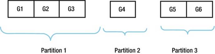
Figure 8-1. Block-range granules on a partitioned table
Figure 8-1 shows how a table with three partitions is split into six block-range granules of roughly equal size even when the partition sizes vary significantly. We could, for example, use two parallel query servers, and each server would probably end up reading data from three of the block-range granules.
![]() Tip When block-range granules are in use the operation PX BLOCK ITERATOR appears in an execution plan. The child of this operation is the object from which the granules are derived.
Tip When block-range granules are in use the operation PX BLOCK ITERATOR appears in an execution plan. The child of this operation is the object from which the granules are derived.
For large tables there are often dozens or even hundreds of granules, with many granules being allocated to each parallel query server.
Let us move on now to the second type of granule—partition granules.
Partition Granules
When a table or an index is partitioned it is possible to allocate partition granules rather than block-range granules. In this case there is exactly one granule per partition (or subpartition). This doesn’t sound like a good idea, as the granules may vary in size significantly, as Figure 8-2 shows:
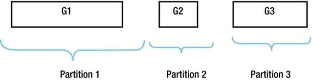
Figure 8-2. Partition granules on a partitioned table
As you can see, there are now only three granules for three partitions, and these granules are all of different sizes. Partition granules can result in some parallel query servers doing most of the work while others lay idle.
![]() Tip When partition granules are in use one of the many operations that begin PX PARTITION ... appears in an execution plan. The child of this operation is the object from which the granules are derived.
Tip When partition granules are in use one of the many operations that begin PX PARTITION ... appears in an execution plan. The child of this operation is the object from which the granules are derived.
There are three main reasons to use partition granules. These are:
· When performing parallel DDL or parallel DML it is often more efficient to have only one parallel query server writing to a partition rather than many.
· As we will see in Chapter 10, it is possible to perform neither an INDEX RANGE SCAN nor an INDEX FULL SCAN on an unpartitioned index in parallel. However, it is possible for one parallel query server to scan one partition of an index while other parallel query servers scan different partitions.
· Partition-wise joins require partition granules. We will cover partition-wise joins in Chapter 11.
Now that we know how data is split up for parallelization, it is time to look at how parallel query servers are organized to enable them access to this granular data.
Data Flow Operators
The Oracle documentation talks about something called a Data Flow Operator, or DFO. Personally, I think that grammatically it should be called a Data Flow Operation, but since I will be using the abbreviation DFO from now on we don’t need to be too worried about this nicety.
A DFO is basically one or more row source operations in an execution plan that form a single unit of parallelized work. To explain this I finally need to show an actual execution plan with a parallel query! Listing 8-20 shows an execution plan with just one DFO.
Listing 8-20. An execution plan with one DFO
CREATE TABLE t5
PARTITION BY HASH (c1)
PARTITIONS 16
AS
SELECT ROWNUM c1, ROWNUM c2
FROM DUAL
CONNECT BY LEVEL <= 10000;
CREATE INDEX t5_i1
ON t5 (c2) local;
SELECT /*+ index(t5) parallel_index(t5) */
*
FROM t5
WHERE c2 IS NOT NULL;
----------------------------------------------------------------------------------------------
| Id | Operation | Name | TQ |IN-OUT| PQ Distrib |
----------------------------------------------------------------------------------------------
| 0 | SELECT STATEMENT | | | | |
| 1 | PX COORDINATOR | | | | |
| 2 | PX SEND QC (RANDOM) | :TQ10000 | Q1,00 | P->S | QC (RAND) |
| 3 | PX PARTITION HASH ALL | | Q1,00 | PCWC | |
| 4 | TABLE ACCESS BY LOCAL INDEX ROWID BATCHED| T5 | Q1,00 | PCWP | |
| 5 | INDEX FULL SCAN | T5_I1 | Q1,00 | PCWP | |
----------------------------------------------------------------------------------------------
Listing 8-20 begins by creating a partitioned table T5 and an associated local index T5_I1. The table is then queried, specifying hints that cause T5 to be accessed by the index. Since block-range granules can’t be used for an INDEX FULL SCAN, you can see the PX PARTITION HASH ALL operation that shows the use of partition granules. Each parallel query server will access one or more partitions and perform operations 4 and 5 on those partitions.
As each parallel query server reads rows from the table, those rows are sent onto the query coordinator (QC) as shown by operation 2. The QC is the original session that existed at the beginning. Apart from receiving the output of the parallel query servers, the QC is also responsible for doling out granules, of whatever type, to the parallel query servers.
Notice the contents of the IN-OUT column in the execution plan. Operation 3 shows PCWC, which means Parallel Combined with Child. Operation 5 shows PCWP, which means Parallel Combined with Parent. Operation 4 is combined with both parent and child. This information can be used to identify the groups of row source operations within each DFO in an execution plan. Incidentally, the IN-OUT column of operation 2 shows P->S, which means Parallel to Serial; the parallel query servers are sending data to the QC.
That wasn’t too difficult to understand, was it? Let me move on to a more complex example that involves multiple DFOs.
Parallel Query Server Sets and DFO Trees
The execution plan in Listing 8-20 involved just one DFO. An execution plan may involve more than one DFO. The set of DFOs is what is referred to as a DFO tree. Listing 8-21 provides an example of a DFO tree with multiple DFOs.
Listing 8-21. Parallel query with multiple DFOs
BEGIN
FOR i IN 1 .. 4
LOOP
DBMS_STATS.gather_table_stats (
ownname => SYS_CONTEXT ('USERENV', 'CURRENT_SCHEMA')
,tabname => 'T' || i);
END LOOP;
END;
/
WITH q1
AS ( SELECT c1, COUNT (*) cnt1
FROM t1
GROUP BY c1)
,q2
AS ( SELECT c2, COUNT (*) cnt2
FROM t2
GROUP BY c2)
SELECT /*+ monitor optimizer_features_enable('11.2.0.3') parallel*/
c1, c2, cnt1
FROM q1, q2
WHERE cnt1 = cnt2;
-----------------------------------------------------------------------------
| Id | Operation | Name | TQ |IN-OUT| PQ Distrib |
-----------------------------------------------------------------------------
| 0 | SELECT STATEMENT | | | | |
| 1 | PX COORDINATOR | | | | |
| 2 | PX SEND QC (RANDOM) | :TQ10003 | Q1,03 | P->S | QC (RAND) |
| 3 | HASH JOIN BUFFERED | | Q1,03 | PCWP | |
| 4 | VIEW | | Q1,03 | PCWP | |
| 5 | HASH GROUP BY | | Q1,03 | PCWP | |
| 6 | PX RECEIVE | | Q1,03 | PCWP | |
| 7 | PX SEND HASH | :TQ10001 | Q1,01 | P->P | HASH |
| 8 | PX BLOCK ITERATOR | | Q1,01 | PCWC | |
| 9 | TABLE ACCESS FULL | T1 | Q1,01 | PCWP | |
| 10 | PX RECEIVE | | Q1,03 | PCWP | |
| 11 | PX SEND BROADCAST | :TQ10002 | Q1,02 | P->P | BROADCAST |
| 12 | VIEW | | Q1,02 | PCWP | |
| 13 | HASH GROUP BY | | Q1,02 | PCWP | |
| 14 | PX RECEIVE | | Q1,02 | PCWP | |
| 15 | PX SEND HASH | :TQ10000 | Q1,00 | P->P | HASH |
| 16 | PX BLOCK ITERATOR | | Q1,00 | PCWC | |
| 17 | TABLE ACCESS FULL| T2 | Q1,00 | PCWP | |
-----------------------------------------------------------------------------
After gathering missing object statistics, Listing 8-21 issues a parallel query. I specified the optimizer_features_enable('11.2.0.3') hint; the 12.1.0.1 plan would have presented some new features somewhat prematurely.
Using the IN-OUT column of Listing 8-21 to identify the DFOs is possible but a little awkward. It is easier to look at the TQ column and see that there are four distinct values reflecting the four DFOs in this plan. We can also look at the operation above each PX SEND operation to see where each DFO is sending its data.
For complex parallel execution plans like this one it is often helpful to draw out the DFO tree. Figure 8-3 shows one way to depict the DFO tree associated with Listing 8-21.
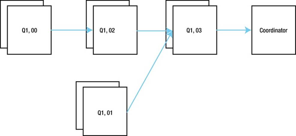
Figure 8-3. Pictorial representation of the DFO tree for Listing 8-21
From Figure 8-3 we can see that three of the four DFOs send data to another DFO, whereas the DFO named Q1, 03 (operations 2 through 6 and operation 10 in the execution plan of Listing 8-21) sends data to the QC.
DFO trees are neither height balanced nor binary; the leaves of the tree are varying distances from the root, and a branch node may have one or several children. The leaves of the tree tend to be operations like full table scans, whereas the branches tend to be joins, aggregations, or sorts.
In order to support multiple concurrent DFOs Oracle database has created the concept of a parallel query server set (PQSS) with each set operating on one DFO at a time. Now, if we had a PQSS for every DFO we would end up with an awful lot of processes for a complex DFO tree. In fact, we only have at most two PQSSs for each DFO tree.
![]() Tip The number of servers in a PQSS is known as the Degree Of Parallelism (DOP), and if there are two PQSSs in a DFO tree the DOP will be the same for both. Furthermore, if you use hints to specify a DOP of 4 for one table and 5 for another, the higher number will normally be used, resulting in the allocation of 10 parallel query servers (although this number may be reduced to conserve resources).
Tip The number of servers in a PQSS is known as the Degree Of Parallelism (DOP), and if there are two PQSSs in a DFO tree the DOP will be the same for both. Furthermore, if you use hints to specify a DOP of 4 for one table and 5 for another, the higher number will normally be used, resulting in the allocation of 10 parallel query servers (although this number may be reduced to conserve resources).
To understand how we can get away with just two PQSSs, it is time to look at how the DFOs communicate with each other and the QC. It is time to introduce table queues.
Table Queues and DFO Ordering
The arrows connecting the nodes in Figure 8-3 represent data being sent from one DFO to another or to the QC. Such communication is facilitated by means of a table queue (TQ). Each table queue has a producer and a consumer. The name of the table queue is shown in the NAME column of the execution plan for PX SEND operations and shows a remarkable similarity to the name of the DFO that is the producer for the TQ. This isn’t a coincidence!
When a producer sends data to a TQ there absolutely must be a consumer actively waiting for that data; don’t let the term queue mislead you into thinking that large amounts of data can be buffered in a TQ. It can’t. I will refer to a TQ as active if a producer and consumer are exchanging data using the TQ. It’s a little odd talking about a piece of memory being active, but I am sure you get the idea.
So how does the runtime engine process this entire DFO tree with just two PQSSs? Well, the runtime engine has to follow a few rules:
1. At any point in time there can be at most one TQ active for a DFO tree.
2. On receipt, the consumer for a TQ must not forward data to another TQ. This is usually accomplished by buffering the data in a workarea.
3. The runtime engine always starts off with :TQ10000 and processes each TQ in numerical order.
Understanding this third rule is the key to reading a parallel execution plan. To quote Jonathan Lewis: Follow the TQs. Let’s use these rules to follow through the sequence of events in Listing 8-21.
The two PQSSs are initially allocated to :TQ10000, one PQSS (let us call it PQSS1) producing and one (let us call it PQSS2) consuming. This means that PQSS1 starts by running DFO Q1, 00 and PQSS2 starts by running Q1, 02. There is a HASH GROUP BY aggregation on line 13 that buffers data so that PQSS2 can comply with rule 2 above. Once all the data from table T2 has been grouped, DFO Q1, 00 is complete. Here is a highlight of the set of operations associated with :TQ10000.
-----------------------------------------------------------------------------
| Id | Operation | Name | TQ |IN-OUT| PQ Distrib |
-----------------------------------------------------------------------------
| 13 | HASH GROUP BY | | Q1,02 | PCWP | |
| 14 | PX RECEIVE | | Q1,02 | PCWP | |
| 15 | PX SEND HASH | :TQ10000 | Q1,00 | P->P | HASH |
| 16 | PX BLOCK ITERATOR | | Q1,00 | PCWC | |
| 17 | TABLE ACCESS FULL| T2 | Q1,00 | PCWP | |
-----------------------------------------------------------------------------
The runtime engine now moves on to :TQ10001. One PQSS starts reading T1 on line 9 (DFO Q1, 01) and sending the data to the other PQSS (DFO Q1, 03). This consuming PQSS groups the data it receives with a HASH GROUP BY operation and then builds a workarea for a hash join. Here is a highlight of the set of operations associated with :TQ10001.
-----------------------------------------------------------------------------
| Id | Operation | Name | TQ |IN-OUT| PQ Distrib |
-----------------------------------------------------------------------------
| 3 | HASH JOIN BUFFERED | | Q1,03 | PCWP | |
| 4 | VIEW | | Q1,03 | PCWP | |
| 5 | HASH GROUP BY | | Q1,03 | PCWP | |
| 6 | PX RECEIVE | | Q1,03 | PCWP | |
| 7 | PX SEND HASH | :TQ10001 | Q1,01 | P->P | HASH |
| 8 | PX BLOCK ITERATOR | | Q1,01 | PCWC | |
| 9 | TABLE ACCESS FULL | T1 | Q1,01 | PCWP | |
-----------------------------------------------------------------------------
At this stage it may not be immediately obvious which PQSS is the producer for :TQ10001 and which is the consumer, but that will soon become clear.
The runtime engine now moves on to :TQ10002. What happens here is that the data from the workarea on line 13 is extracted and then sent from one PQSS to another. Here is a highlight of the set of operations associated with :TQ10002.
-----------------------------------------------------------------------------
| Id | Operation | Name | TQ |IN-OUT| PQ Distrib |
-----------------------------------------------------------------------------
| 3 | HASH JOIN BUFFERED | | Q1,03 | PCWP | |
< lines not involved cut> |
| 10 | PX RECEIVE | | Q1,03 | PCWP | |
| 11 | PX SEND BROADCAST | :TQ10002 | Q1,02 | P->P | BROADCAST |
| 12 | VIEW | | Q1,02 | PCWP | |
| 13 | HASH GROUP BY | | Q1,02 | PCWP | |
-----------------------------------------------------------------------------
The final TQ in our DFO tree is :TQ10003, but let us pause briefly before looking at that in detail.
We always use the same PQSS for all operations in a DFO, so the producer for :TQ10002 must be PQSS2 as PQSS2 ran Q1, 02 when Q1, 02 was the consumer for :TQ10000. This, in turn, means that the consumer for :TQ10002 is PQSS1, and as this is DFO Q1, 03, we can work backwards and conclude that the consumer for :TQ10001 must also have been PQSS1 and that the producer for :TQ10001 must have been PQSS2. If your head is spinning a bit from this explanation take another look at Figure 8-3. Any two adjacent nodes in the DFO tree must use different PQSSs, and so after allocating PQSS1 to DFO Q1, 00 there is only one way to allocate PQSSs to the remaining DFOs.
You can now see that PQSS1 runs Q1, 00 and Q1, 03 and that PQSS2 runs Q1, 01 and Q1, 02. You can confirm this analysis if you produce a SQL Monitor report (despite the fact that the query ran almost instantly, this report is available due to the MONITOR hint in Listing 8-21) using one of the scripts shown in Listing 4-6. Figure 8-4 shows a snippet from the report.
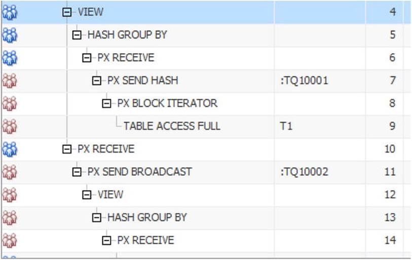
Figure 8-4. Snippet from SQL Monitor report showing relationship of DFO and Parallel Query Server Sets
Figure 8-4 shows PQSS1 by three blue people (dark gray in the absence of color) in a huddle and PQSS2 as three pink people (light gray in the absence of color).
This is all very tricky, so let me walk through DFO Q1, 02 and DFO Q1, 03 again. Each member of PQSS2 builds a workarea associated with the HASH GROUP BY on line 13 when acting as the consumer for :TQ10000. DFO Q1,02 is then effectively suspended while :TQ10001 is active. PQSS2 resumes DFO Q1,02, this time acting as a producer, when :TQ10002 becomes active and reads the data from the workarea.
Rule 2 above states that the consumer of a TQ cannot forward the data to another TQ. Yet—on receipt of the data on line 10—it looks like the second part of the hash join on line 3 will start producing rows and sending them to the coordinator on line 2. Isn’t this a violation of rule 2? It looks like :TQ10002 and :TQ10003 will both be active at the same time. The clue, as you might have guessed, comes from the word BUFFERED in line 3. In actual fact, the data from line 10 is not joined at this point—it is just buffered. I will provide a more detailed explanation of theHASH JOIN BUFFERED operation in Chapter 11 when I cover joins in more detail.
Once all the data has been sent from PQSS2 to PQSS1 and buffered, PQSS1 moves on to :TQ10003. PQSS1 can now read the data that it just buffered, perform the join on line 3, and send the data to the QC. Here are the steps associated with :TQ10003:
-----------------------------------------------------------------------------
| Id | Operation | Name | TQ |IN-OUT| PQ Distrib |
-----------------------------------------------------------------------------
| 1 | PX COORDINATOR | | | | |
| 2 | PX SEND QC (RANDOM) | :TQ10003 | Q1,03 | P->S | QC (RAND) |
| 3 | HASH JOIN BUFFERED | | Q1,03 | PCWP | |
-----------------------------------------------------------------------------
To recap:
· Rows are placed into the workarea of the HASH GROUP BY on line 13 when :TQ10000 is active and those rows are extracted when :TQ10002 is active.
· Rows are placed into the in-memory hash cluster of the HASH JOIN BUFFERED operation on line 3 when :TQ10001 is active, rows for the probe row source are buffered when :TQ10002 is active, and the actual join is performed when :TQ10003 is active.
Now you might have a question at this point. It usually makes sense to have only one TQ active at once, otherwise a PQSS might have to produce on one TQ and consume from another simultaneously. However, in the case of :TQ10002 and :TQ10003 the restriction seems unnecessary. Why can’t PQSS2 send data to PQSS1, which then would simply forward the results of the join to the QC? Many of us would like to know. Perhaps one day Oracle will either tell us the reason or remove the restriction from both the CBO and the runtime engine. In the meantime, we can only speculate.
Multiple DFO Trees
Listing 8-21 only had one DFO tree, and all DFOs were processed by a PQSS. Unfortunately, some SQL statements require more than one DFO tree, and sometimes a DFO is processed by the QC. Listing 8-22 demonstrates these points.
Listing 8-22. Parallel query with multiple DFO trees
COMMIT;
ALTER SESSION DISABLE PARALLEL DML;
WITH q1
AS ( SELECT /*+
parallel(T1)
full(t1)
no_parallel(t2)
no_pq_replicate(t2)
no_gby_pushdown
pq_distribute(t2 none broadcast)
*/
c1 + c2 c12, AVG (c1) avg_c1, COUNT (c2) cnt_c2
FROM t1, t2
WHERE c1 = c2 + 1
GROUP BY c1 + c2
ORDER BY 1)
,q2 AS (SELECT ROWNUM rn, c12 FROM q1)
SELECT /*+ leading(q1)
pq_distribute(q2 none broadcast) */
*
FROM q1 NATURAL JOIN q2
ORDER BY cnt_c2;
-----------------------------------------------------------------------------------------
| Id | Operation | Name | TQ |IN-OUT| PQ Distrib |
-----------------------------------------------------------------------------------------
| 0 | SELECT STATEMENT | | | | |
| 1 | TEMP TABLE TRANSFORMATION | | | | |
| 2 | PX COORDINATOR | | | | |
| 3 | PX SEND QC (RANDOM) | :TQ10002 | Q1,02 | P->S | QC (RAND) |
| 4 | LOAD AS SELECT | SYS_TEMP_0FD9D6| Q1,02 | PCWP | |
| 5 | SORT GROUP BY | | Q1,02 | PCWP | |
| 6 | PX RECEIVE | | Q1,02 | PCWP | |
| 7 | PX SEND RANGE | :TQ10001 | Q1,01 | P->P | RANGE |
| 8 | HASH JOIN BUFFERED | | Q1,01 | PCWP | |
| 9 | PX BLOCK ITERATOR | | Q1,01 | PCWC | |
| 10 | TABLE ACCESS FULL | T1 | Q1,01 | PCWP | |
| 11 | PX RECEIVE | | Q1,01 | PCWP | |
| 12 | PX SEND BROADCAST | :TQ10000 | Q1,00 | S->P | BROADCAST |
| 13 | PX SELECTOR | | Q1,00 | SCWC | |
| 14 | TABLE ACCESS FULL | T2 | Q1,00 | SCWP | |
| 15 | PX COORDINATOR | | | | |
| 16 | PX SEND QC (ORDER) | :TQ20003 | Q2,03 | P->S | QC (ORDER) |
| 17 | SORT ORDER BY | | Q2,03 | PCWP | |
| 18 | PX RECEIVE | | Q2,03 | PCWP | |
| 19 | PX SEND RANGE | :TQ20002 | Q2,02 | P->P | RANGE |
| 20 | HASH JOIN BUFFERED | | Q2,02 | PCWP | |
| 21 | VIEW | | Q2,02 | PCWP | |
| 22 | PX BLOCK ITERATOR | | Q2,02 | PCWC | |
| 23 | TABLE ACCESS FULL | SYS_TEMP_0FD9D6| Q2,02 | PCWP | |
| 24 | PX RECEIVE | | Q2,02 | PCWP | |
| 25 | PX SEND BROADCAST | :TQ20001 | Q2,01 | S->P | BROADCAST |
| 26 | BUFFER SORT | | Q2,01 | SCWP | |
| 27 | VIEW | | Q2,01 | SCWC | |
| 28 | COUNT | | Q2,01 | SCWP | |
| 29 | PX RECEIVE | | Q2,01 | SCWP | |
| 30 | PX SEND 1 SLAVE | :TQ20000 | Q2,00 | P->S | 1 SLAVE |
| 31 | VIEW | | Q2,00 | PCWP | |
| 32 | PX BLOCK ITERATOR | | Q2,00 | PCWC | |
| 33 | TABLE ACCESS FULL| SYS_TEMP_0FD9D6| Q2,00 | PCWP | |
-----------------------------------------------------------------------------------------
Don’t worry about what the query in Listing 8-22 does. Focus on the execution plan instead. The first thing to look at is operation 4. The LOAD AS SELECT has a value of PCWP (Parallel Combined with Child) in the IN-OUT column, clearly showing that we are loading a table in parallel. This may surprise you because Listing 8-22 begins by disabling parallel DML. But the purpose of disabling parallel DML is to prevent the ORA-12838 error, as in Listing 8-19. Since the temporary table we are loading has been created for materializing the factored subquery Q1 and will cease to exist at the end of this statement, such an error is impossible; we can use parallel DML even though it is ostensibly disabled.
Next look at operations 12, 13, and 14. These operations read table T2 serially, as you can see from the IN-OUT column values. The PX SELECTOR operation on line 13 is new to 12cR1 and indicates that the serial operation is done by a parallel query server from PQSS1 and not by the QC as in earlier releases. Line 12 shows that all selected rows from T2 are broadcast to all members of PQSS2. We will look at other ways that parallel query servers can communicate with each other shortly.
Now take a look at the operation on line 30. There are two things to notice about this operation. First, the newly created temporary table is read in parallel by PQSS1 (I have truncated the table name to save space on the page), but all rows are sent to a single member of PQSS2, as suggested by the operation name and confirmed by the IN-OUT column. All rows are processed by one slave in PQSS2 because of the use of the ROWNUM pseudo-column in the query. Once again, the PX SEND 1 SLAVE operation is new to 12cR1, and in prior releases this operation would have been PX SEND QC (RANDOM), as the COUNT operation that implements the ROWNUM pseudo-column would have been performed by the QC.
The second thing to note about operation 30 is that the name of the DFO is Q2, 00 and the TQ name is :TQ20000. These names show that a second DFO tree is used in the statement, and all lines from 16 to 33 are performed by this second DFO tree. When multiple DFO trees are involved in a statement each DFO tree usually gets its own parallel query server set or its own pair of parallel query server sets, and indeed the DOP may differ from one DFO tree to the next. The parallel query server sets that support a particular DFO tree are known as a parallel group. So in the case of Listing 8-22 there are a total of four parallel query slave server sets—two sets per group.
Finally, I want to turn your attention to operation 26. Do you recall that a consumer from a TQ must buffer its data? On line 3 in Listing 8-21 and on line 20 in Listing 8-22 this buffering is incorporated into the HASH JOIN BUFFERED operation, but on line 26 in Listing 8-22 the buffering is a separate and explicit operation. Don’t worry about the word sort. This is one of numerous cases where the BUFFER SORT operation doesn’t sort.
Parallel Query Distribution Mechanisms
Listings 8-21 and 8-22 use the PX SEND HASH, PX SEND RANGE, PX SEND BROADCAST, PX SEND QC (RANDOM), and PX_SEND QC (ORDER) operations. These myriad ways in which producers send data through table queues reflect the variety of data distribution mechanisms with which these operations are associated. It is now time to explain these distribution mechanisms. We will begin with data-loading distribution mechanisms for partitioned tables and then move on to the distribution mechanisms associated with joins and other operations.
Data-loading Distribution Mechanisms for Partitioned Tables
Although there have been a number of data-loading distribution mechanisms available for some time, they were only documented in the context of the hints that control them in 11gR2. In this section I will discuss just two data-loading distribution mechanisms that can be used when loading data into multiple partitions of a partitioned table. For further information you can consult the description of the PQ_DISTRIBUTE hint in the SQL Reference Manual.
Imagine you are loading data into a hash partitioned table with eight partitions. The natural thing to do would be to have one parallel query server per partition of the table being loaded, wouldn’t it? Yes, it would! Listing 8-23 demonstrates.
Listing 8-23. Loading data with no skew into a hash partitioned table
CREATE TABLE t_part1
PARTITION BY HASH (c1)
PARTITIONS 8
AS
SELECT c1, ROWNUM AS c3 FROM t1;
CREATE TABLE t_part2
PARTITION BY HASH (c2)
PARTITIONS 8
AS
SELECT c1 AS c2, ROWNUM AS c4 FROM t1;
ALTER SESSION ENABLE PARALLEL DML;
INSERT /*+ parallel(t_part1 8) pq_distribute(t_part1 PARTITION)*/
INTO t_part1
SELECT c1,c1 FROM t1;
------------------------------------------------------------------------------------
| Id | Operation | Name | TQ |IN-OUT| PQ Distrib |
------------------------------------------------------------------------------------
| 0 | INSERT STATEMENT | | | | |
| 1 | PX COORDINATOR | | | | |
| 2 | PX SEND QC (RANDOM) | :TQ10001 | Q1,01 | P->S | QC (RAND) |
| 3 | LOAD AS SELECT | T_PART1 | Q1,01 | PCWP | |
| 4 | OPTIMIZER STATISTICS GATHERING | | Q1,01 | PCWP | |
| 5 | PX RECEIVE | | Q1,01 | PCWP | |
| 6 | PX SEND PARTITION (KEY) | :TQ10000 | Q1,00 | S->P | PART (KEY) |
| 7 | PX SELECTOR | | Q1,00 | SCWC | |
| 8 | TABLE ACCESS FULL | T1 | Q1,00 | SCWP | |
------------------------------------------------------------------------------------
After creating a couple of partitioned tables and enabling parallel DML, Listing 8-23 copies data from one unpartitioned table into a partitioned table using one loading server per partition. We have used hints to demonstrate how to force this loading technique. In this case, the unpartitioned table T1 is read serially; each row is then sent to whichever parallel query slave is responsible for loading data into the partition for which the row is destined.
That seems all well and good, but what if most of the data you are reading goes into just one or two partitions? Having just one process writing to a partition won’t help much. Take a look at Listing 8-24.
Listing 8-24. Loading data with skew into a hash partitioned table
INSERT /*+ parallel(t_part1 8) pq_distribute(t_part1 RANDOM) */
INTO t_part1
SELECT /*+ parallel(t_part2 8) */ * FROM t_part2;
------------------------------------------------------------------------------------
| Id | Operation | Name | TQ |IN-OUT| PQ Distrib |
------------------------------------------------------------------------------------
| 0 | INSERT STATEMENT | | | | |
| 1 | PX COORDINATOR | | | | |
| 2 | PX SEND QC (RANDOM) | :TQ10001 | Q1,01 | P->S | QC (RAND) |
| 3 | LOAD AS SELECT | T_PART1 | Q1,01 | PCWP | |
| 4 | OPTIMIZER STATISTICS GATHERING | | Q1,01 | PCWP | |
| 5 | PX RECEIVE | | Q1,01 | PCWP | |
| 6 | PX SEND ROUND-ROBIN | :TQ10000 | Q1,00 | S->P | RND-ROBIN |
| 7 | PARTITION HASH ALL | | | | |
| 8 | TABLE ACCESS FULL | T_PART2 | | | |
------------------------------------------------------------------------------------
The data-loading mechanism used in Listing 8-24 will be most effective when most data is targeted for one or two partitions as each server can load data into all partitions. Because of the way direct path writes work, this would be inefficient when rows are evenly distributed among partitions.
Correlated Subquery Distribution Mechanisms
Prior to 12cR1 the evaluation of correlated subqueries that could not be unnested was either done serially or by an entirely separate DFO tree. 12cR1 introduced several ways in which correlated subqueries could be evaluated in parallel. It also introduced the PQ_FILTER hint to give you some control over that mechanism. Listing 8-25 shows two of four options.
Listing 8-25. Parallel execution of correlated subquery evaluation
SELECT /*+ SELECT /*+
parallel(t1) full(t1) parallel(t1) full(t1)
pq_filter(NONE) pq_filter(HASH)
*/ */
* *
FROM t1 FROM t1
WHERE EXISTS WHERE EXISTS
(SELECT null (SELECT null
FROM t2 FROM t2
WHERE t1.c1 != t2.c2); WHERE t1.c1 != t2.c2);
------------------------------------------ ---------------------------------------------
| Id | Operation | Name | | Id | Operation | Name |
------------------------------------------ ---------------------------------------------
| 0 | SELECT STATEMENT | | | 0 | SELECT STATEMENT | |
| 1 | PX COORDINATOR | | | 1 | PX COORDINATOR | |
| 2 | PX SEND QC (RANDOM) | :TQ10000 | | 2 | PX SEND QC (RANDOM) | :TQ10001 |
| 3 | FILTER | | | 3 | BUFFER SORT | |
| 4 | PX BLOCK ITERATOR | | | 4 | FILTER | |
| 5 | TABLE ACCESS FULL| T1 | | 5 | PX RECEIVE | |
| 6 | TABLE ACCESS FULL | T2 | | 6 | PX SEND HASH | :TQ10000 |
------------------------------------------ | 7 | PX BLOCK ITERATOR | |
| 8 | TABLE ACCESS FULL| T1 |
| 9 | TABLE ACCESS FULL | T2 |
---------------------------------------------
The query in Listing 8-25 reads T1 in parallel and filters the results using a correlated subquery, which cannot be unnested.
Suppose that T1 is huge, the evaluation of the correlated subquery is cheap, and the filter gets rid of most of the rows from T1. In that case, the PQ_FILTER (NONE) hint on left-hand side would be a good idea, as the resulting execution plan evaluates the subquery with the same parallel query server that reads T1, and there is only one DFO; we don’t send all the unfiltered data through a TQ. This is probably the most sensible approach in most cases.
On the other hand, suppose that T1 isn’t that big but the calculations performed by the correlated subquery are very expensive. In that case, you can arrange for the filtering to be done by a separate DFO concurrently with the parallelized full table scan of T1. This is accomplished by the use of the PQ_FILTER (HASH) hint on the right-hand side of Listing 8-25.
The execution plan on the right-hand side of Listing 8-25 shows that as PQSS1 reads rows from T1 it sends them to a member of PQSS2 based on a hash of T1.C1. Note that the presence of the second DFO means that data needs to be buffered after filtering before sending data to the QC, and, at the risk of sounding repetitive, I want to remind you again that there is no sort involved in operation 3 despite appearances.
There are two more legal values for the PQ_FILTER hint parameter. PQ_FILTER (SERIAL) causes all correlated subquery evaluations to be performed by the QC as with 11gR2 and earlier. Having the QC perform filtering might be a good idea if the number of distinct values of the correlated column T1.C1 is low, as scalar subquery caching may prevent the subquery from being evaluated repeatedly.
If you specify the PQ_FILTER (RANDOM) hint, rows are sent from PQSS1 to PQSS2 on a round-robin basis rather than based on a hash function on T1.C1, as with the PQ_FILTER (HASH) distribution mechanism. According to the documentation, this distribution mechanism should be used when there is skew in the data, but this makes no sense to me. Suppose all the rows in T1 had exactly the same value for T1.C1. The PX SEND HASH operation shown on line 6 of the execution plan on the right-hand side of Listing 8-25 would send all the rows to the same member of PQSS2, but scalar subquery caching would prevent the multiple evaluations of the subquery that would arise with PQ_FILTER (RANDOM).
Subqueries that can’t be unnested are a rarity these days, and the occasions when they need to be evaluated in parallel are even rarer. I must confess that I have no practical experience with this 12cR1 feature; the above analysis is purely theoretical and could be flawed. At least now you know as much as I do!
Other Parallel Distribution Mechanisms
The PQ_DISTRIBUTE hint isn’t used only to control different approaches to loading data. In fact, by far the most common use of this hint is to control the different approaches for joining tables in parallel. I will cover these distribution mechanisms in Chapter 11 once I have covered the different methods for joining tables serially.
There are one or two other ways that a producing PQSS can distribute its data through a TQ, but these are for specific situations and there is no choice of distribution mechanism; the PQ_DISTRIBUTE hint is neither legal nor required.
For example, you will see the PX SEND RANGE operation on line 7 in Listing 8-22. This is because the consumer of the TQ performs a sort in parallel. Chapter 17 is dedicated to sorts; we will take a look at the parallelization of sorts there. The same listing shows a PX SEND QC (RANDOM) operation on line 3 and a PX SEND QC (ORDER) operation on line 16. Both distribution mechanisms involve sending data to the QC, but in the former case the order in which members of the PQSS send data to the QC is of no relevance—the PQSS members just notify the QC that they have finished loading data and the QC just wants to know when everything is done. In the latter case the order in which the PQSS members send rows to the QC is important because the final result set needs to be ordered by CNT_C2.
Why Forcing Parallel Query Doesn’t Force Parallel Query
The PARALLEL and PARALLEL_INDEX hints are used to authorize the CBO to use parallel execution to perform operations in parallel and optionally to specify the DOP to be used. However, if the CBO has the choice to use an operation that cannot be performed in parallel, such as an index range scan, then it may elect to choose that access method and run it serially rather than use an alternative, more expensive, parallel operation.
The statement ALTER SESSION FORCE PARALLEL QUERY essentially adds PARALLEL and PARALLEL_INDEX statement-level hints to each SQL statement in the session; Listing 8-26 demonstrates that parallel execution isn’t guaranteed by the statement.
Listing 8-26. Understanding FORCE PARALLEL QUERY
ALTER SESSION FORCE PARALLEL QUERY PARALLEL 2;
SELECT *
FROM sh.customers c
WHERE cust_id < 100;
-------------------------------------------------------------------------
| Id | Operation | Name | Cost (%CPU)|
-------------------------------------------------------------------------
| 0 | SELECT STATEMENT | | 54 (0)|
| 1 | TABLE ACCESS BY INDEX ROWID BATCHED| CUSTOMERS | 54 (0)|
|* 2 | INDEX RANGE SCAN | CUSTOMERS_PK | 2 (0)|
-------------------------------------------------------------------------
Predicate Information (identified by operation id):
---------------------------------------------------
2 - access("CUST_ID"<100)
SELECT /*+ full(c)*/
*
FROM sh.customers c
WHERE cust_id < 100;
-------------------------------------------------------
| Id | Operation | Name | Cost (%CPU)|
-------------------------------------------------------
| 0 | SELECT STATEMENT | | 235 (1)|
| 1 | PX COORDINATOR | | |
| 2 | PX SEND QC (RANDOM)| :TQ10000 | 235 (1)|
| 3 | PX BLOCK ITERATOR | | 235 (1)|
|* 4 | TABLE ACCESS FULL| CUSTOMERS | 235 (1)|
-------------------------------------------------------
Predicate Information (identified by operation id):
---------------------------------------------------
4 - filter("CUST_ID"<100)
ALTER SESSION FORCE PARALLEL QUERY PARALLEL 20;
SELECT *
FROM sh.customers c
WHERE cust_id < 100;
-------------------------------------------------------
| Id | Operation | Name | Cost (%CPU)|
-------------------------------------------------------
| 0 | SELECT STATEMENT | | 23 (0)|
| 1 | PX COORDINATOR | | |
| 2 | PX SEND QC (RANDOM)| :TQ10000 | 23 (0)|
| 3 | PX BLOCK ITERATOR | | 23 (0)|
|* 4 | TABLE ACCESS FULL| CUSTOMERS | 23 (0)|
-------------------------------------------------------
Predicate Information (identified by operation id):
---------------------------------------------------
4 - filter("CUST_ID"<100)
ALTER SESSION ENABLE PARALLEL QUERY;
Listing 8-26 begins by “forcing” a DOP of two before querying the SH.CUSTOMERS table. The resultant execution plan uses an index range scan that is run serially with a cost of 54. When I force a full table scan with a hint, you can see that the CBO elects to run it in parallel, but the cost of 235 is much higher than the alternative serial index range scan. However, the final query in Listing 8-26 runs with a DOP of 20. Now the cost of the parallel full table scan is 23 because each parallel query slave now has fewer blocks to read; the CBO calculates that the parallel query operation will now complete quicker than the equivalent index range scan.
In Chapter 10 we will look at the index range scan in more detail and it will become clear why block-range granules cannot be used to run an index range scan in parallel.
Further Reading
There is a lot more to the topic of parallel execution than I have covered in this chapter. There are several initialization parameters that control such things as the minimum and maximum number of parallel execution slaves that an instance can support. There are features such as statement queuing and DOP downgrade that determine what happens when the desired number of parallel query servers aren’t available. You can also the use the resource manager to prioritize parallel execution. For details on all of these features and information about the views that can be used to monitor parallel execution, I repeat my recommendation to take a look at the VLDB and Partitioning Guide.
That concludes our discussion on parallel execution. It is time to move on to the third and final major topic of this chapter: global hints.
Understanding Global Hints
The vast majority of embedded hints in SQL statements are local hints, meaning that they apply to the query block in which they are placed. In an outline, all the hints for all query blocks are placed in one place and so some way has to be found to indicate the query block to which each hint applies. This is accomplished by means of an ‘@’ symbol as the leading character of the first argument to the hint, marking it as global. Take a look at lines 4, 8, and 12 in Listing 8-7. These are all LEADING hints, but line 4 applies to the query block SEL$F1D6E378, which as I explained earlier is the query block formed by the merge of query blocks SEL$1 into SEL$3, whereas the hints on lines 8 and 12 apply to query blocks SEL$2 and SEL$4, respectively.
Global hints are documented in the SQL Language Reference manual, are fully supported when embedded in SQL statements, and are often invaluable. There are at least three types of occasions that warrant the use of global hints, seen here:
· You want to hint a block originating in a data dictionary view. To use a local hint in this case would require the definition of the view to be altered and would affect other users of the view.
· You want to hint a query block that is the result of a query transformation. In these cases local hints can be confusing to the reader.
· Where hints are so numerous that they impair the readability of the original statement, global hints allow them all to be collected in one place.
I will provide simple examples of the first two scenarios, but providing a simple example of complex hinting is somewhat of an oxymoron. After demonstrating these scenarios I will focus in on the NO_MERGE hint, as the multiple variants of this very common hint are somewhat daunting. If you can grasp the NO_MERGE hint you can consider yourself a master of global hinting!
Hinting Data Dictionary Views
Listing 8-27 creates a data dictionary view and uses that view in a query. To keep things simple, I also drop the index on T1 and disable parallel query.
Listing 8-27. Simple query using a data dictionary view
ALTER SESSION DISABLE PARALLEL QUERY;
DROP INDEX t1_i1
CREATE OR REPLACE VIEW v1
AS
SELECT c1, MEDIAN (c2) med_c2
FROM t1, t2
WHERE t1.c1 = t2.c2
GROUP BY t1.c1;
SELECT *
FROM v1, t3
WHERE v1.c1 = t3.c3;
Plan hash value: 808098385
--------------------------------------
| Id | Operation | Name |
--------------------------------------
| 0 | SELECT STATEMENT | |
| 1 | HASH JOIN | |
| 2 | VIEW | V1 |
| 3 | HASH GROUP BY | |
| 4 | HASH JOIN | |
| 5 | TABLE ACCESS FULL| T1 |
| 6 | TABLE ACCESS FULL| T2 |
| 7 | TABLE ACCESS FULL | T3 |
--------------------------------------
Query Block Name / Object Alias (identified by operation id):
-------------------------------------------------------------
1 - SEL$1
2 - SEL$2 / V1@SEL$1
3 - SEL$2
5 - SEL$2 / T1@SEL$2
6 - SEL$2 / T2@SEL$2
7 - SEL$1 / T3@SEL$1
Outline Data
-------------
/*+
BEGIN_OUTLINE_DATA
USE_HASH_AGGREGATION(@"SEL$2")
USE_HASH(@"SEL$2" "T2"@"SEL$2")
LEADING(@"SEL$2" "T1"@"SEL$2" "T2"@"SEL$2")
FULL(@"SEL$2" "T2"@"SEL$2")
FULL(@"SEL$2" "T1"@"SEL$2")
USE_HASH(@"SEL$1" "T3"@"SEL$1")
LEADING(@"SEL$1" "V1"@"SEL$1" "T3"@"SEL$1")
FULL(@"SEL$1" "T3"@"SEL$1")
NO_ACCESS(@"SEL$1" "V1"@"SEL$1")
OUTLINE_LEAF(@"SEL$1")
OUTLINE_LEAF(@"SEL$2")
ALL_ROWS
DB_VERSION('12.1.0.1')
OPTIMIZER_FEATURES_ENABLE('12.1.0.1')
IGNORE_OPTIM_EMBEDDED_HINTS
END_OUTLINE_DATA
*/
Now imagine that you wish to change the HASH JOIN of T1 and T2 to a nested loops join driven by T1. Of course, this doesn’t make sense from a performance perspective, but I am just trying to explain the principle with a simple example at this point. Listing 8-28 shows how to do this without editing the view definition.
Listing 8-28. Applying a hint to a query block embedded in a data dictionary view
SELECT
/*+
LEADING(@"SEL$2" "T1"@"SEL$2" "T2"@"SEL$2")
USE_NL(@"SEL$2" "T2"@"SEL$2")
*/
*
FROM v1, t3
WHERE v1.c1 = t3.c3;
Plan hash value: 1369664419
--------------------------------------
| Id | Operation | Name |
--------------------------------------
| 0 | SELECT STATEMENT | |
| 1 | HASH JOIN | |
| 2 | VIEW | V1 |
| 3 | HASH GROUP BY | |
| 4 | NESTED LOOPS | |
| 5 | TABLE ACCESS FULL| T1 |
| 6 | TABLE ACCESS FULL| T2 |
| 7 | TABLE ACCESS FULL | T3 |
--------------------------------------
Query Block Name / Object Alias (identified by operation id):
-------------------------------------------------------------
1 - SEL$1
2 - SEL$2 / V1@SEL$1
3 - SEL$2
5 - SEL$2 / T1@SEL$2
6 - SEL$2 / T2@SEL$2
7 - SEL$1 / T3@SEL$1
Outline Data
-------------
/*+
BEGIN_OUTLINE_DATA
USE_HASH_AGGREGATION(@"SEL$2")
USE_NL(@"SEL$2" "T2"@"SEL$2")
LEADING(@"SEL$2" "T1"@"SEL$2" "T2"@"SEL$2")
FULL(@"SEL$2" "T2"@"SEL$2")
FULL(@"SEL$2" "T1"@"SEL$2")
USE_HASH(@"SEL$1" "T3"@"SEL$1")
LEADING(@"SEL$1" "V1"@"SEL$1" "T3"@"SEL$1")
FULL(@"SEL$1" "T3"@"SEL$1")
NO_ACCESS(@"SEL$1" "V1"@"SEL$1")
OUTLINE_LEAF(@"SEL$1")
OUTLINE_LEAF(@"SEL$2")
ALL_ROWS
DB_VERSION('12.1.0.1')
OPTIMIZER_FEATURES_ENABLE('12.1.0.1')
IGNORE_OPTIM_EMBEDDED_HINTS
END_OUTLINE_DATA
*/
What I did here was to look at the highlighted lines from the ALIAS and OUTLINE sections of the execution plan for the original statement in Listing 8-27 to determine the correct query block name and object aliases to use. Since a query block isn’t listed for operation 4, I could determine the correct query block by looking at the query block for operation 3. I then used that information to construct suitable global hints to embed in my SQL statement. The execution plan for the statement in Listing 8-28 shows that the hints had the desired result.
![]() Note It is important to realize that, unlike local hints, the place that global hints appear is irrelevant; they can be placed in any legal location in a SQL statement and the effect will be the same.
Note It is important to realize that, unlike local hints, the place that global hints appear is irrelevant; they can be placed in any legal location in a SQL statement and the effect will be the same.
Applying Hints to Transformed Queries
Generally speaking, local hints are preferable to global hints as they are easier for a reader to understand, but this isn’t always the case. In Chapter 13 of this book I will discuss the star transformation and subquery unnesting transformation. These two transformations, amongst others, can result in an execution plan that seems to bear little resemblance to the original SQL statement, and local hints seem meaningless. Even when there have been few, if any, transformations, there comes a point where large numbers of local hints scattered around a complex statement become impediments to the readability of the original code. In these hopefully rare cases, a single block of global hints can, in my opinion, make understanding the statement and its associated hints easier. Providing a simple example of obfuscation is a bit of a challenge, but Listing 8-29 might just help make my point.
Listing 8-29. Local hints applied to an unnested subquery
SELECT *
FROM t1
WHERE NOT EXISTS
(SELECT /*+ unnest use_nl(t2)*/
1
FROM t2
WHERE t2.c2 = t1.c1);
I have deliberately withheld the execution plan for Listing 8-29 in order to simulate the experience of the programmer reading through source code. The USE_NL hint controls join mechanism and seems meaningless as it appears in a block that contains only one row source. Nevertheless, this hint is valid because it is applied to a transformed block that contains multiple row sources. Since these hints only make sense when looking at the transformed execution plan, it is surely best to group all such hints in one place so that the business logic remains uncluttered.
The NO_MERGE Hint
I would like to conclude this discussion of global hints with a note about the MERGE and NO_MERGE hints. When used as local hints, the MERGE and NO_MERGE hints have two variants. Both local variants have equivalent global forms, thus making a total of four variants. It is easy to confuse these four variants, so let me clear things up. For simplicity I will stick to the NO_MERGE hint, as it is by far the more common embedded hint.
· When used as a local hint with no arguments, NO_MERGE instructs the CBO not to merge the query block in which the hint appears.
· When used as a local hint with one argument (not preceded by an ‘@’ symbol), that argument is assumed to be a data dictionary view, a factored subquery, or an inline view. The NO_MERGE hint instructs the CBO not to merge the row source named in the argument.
· When used as a global hint with one argument preceded by an ‘@’ symbol, the NO_MERGE hint instructs the CBO not to merge the query block named in the argument.
· When used as a global hint with two arguments (the first preceded by an ‘@’ symbol), the second argument is assumed to be a data dictionary view, a factored subquery, or an inline view appearing in the query block specified by the first argument. The NO_MERGE hint instructs the CBO not to merge the row source named in the second argument that appears in the query block specified in the first argument.
Confused? Perhaps Listing 8-30 can shed some light.
Listing 8-30. The four variants of the NO_MERGE hint
WITH fs AS (SELECT /*+ qb_name(qb1) no_merge*/
* FROM t1)
SELECT /*+ qb_name(qb2) */
*
FROM fs myalias, t2
WHERE myalias.c1 = t2.c2;
WITH fs AS (SELECT /*+ qb_name(qb1) */
* FROM t1)
SELECT /*+ qb_name(qb2) no_merge(myalias)*/
*
FROM fs myalias, t2
WHERE myalias.c1 = t2.c2;
WITH fs AS (SELECT /*+ qb_name(qb1) */
* FROM t1)
SELECT /*+ qb_name(qb2) no_merge(@qb1)*/
*
FROM fs myalias, t2
WHERE myalias.c1 = t2.c2;
WITH fs AS (SELECT /*+ qb_name(qb1) no_merge(@qb2 myalias)*/
* FROM t1)
SELECT /*+ qb_name(qb2) */
*
FROM fs myalias, t2
WHERE myalias.c1 = t2.c2;
Plan hash value: 2191810965
------------------------------------
| Id | Operation | Name |
------------------------------------
| 0 | SELECT STATEMENT | |
| 1 | HASH JOIN | |
| 2 | VIEW | |
| 3 | TABLE ACCESS FULL| T1 |
| 4 | TABLE ACCESS FULL | T2 |
------------------------------------
With the exception of hints, the four statements in Listing 8-30 are identical. They all contain two query blocks that would be merged unless a hint prevented it. Each of the four statements contains one NO_MERGE hint that succeeds in preventing the merge, but these four hints are subtly different.
The key to understanding how the hints operate is to understand the three different ways by which the first query block is named.
· FS is the name of the factored subquery and allows the main query to reference it just like a table.
· QB1 is the name of the query block. This has been assigned by the QB_NAME hint and is relevant only for global hints.
· MYALIAS is an object alias assigned in the FROM clause of the main query. Its primary purpose is to qualify the names of columns in the main query block, but it also has uses in the NO_MERGE hint. The existence of an object alias renders further reference to the identifier FS illegal.
With this in mind let us look at the four hints in turn.
· In the first query the NO_MERGE hint has no arguments. It is a local hint that instructs the CBO not to merge the block in which the hint appears. Like any local hint, it must be placed in the block to which it applies, in this case the subquery.
· The second query also uses a local NO_MERGE hint, but this time an argument is supplied. The argument specifies the object alias of the row source that must not be merged. Accordingly, the correct argument value is MYALIAS. Like any local hint, it must be placed in the block to which it applies, in this case the main query because the row source appears in the FROM clause of the main query.
· The third variant uses global hint syntax. The supplied query block name QB1 indicates that the hint should operate like a local hint in QB1. There being no other argument apart from the query block name, the hint operates just like the first variant with the exception that the hint can appear anywhere in the statement.
· The fourth variant is also a global hint. The supplied query block name QB2 indicates that the hint should operate like a local hint placed in QB2. The second argument in the fourth variant, MYALIAS, is treated like the first argument in the second variant. Like any global hint, its location in the statement is irrelevant—the hint always operates on the main query block QB2.
Are you scratching your head at this point? Don’t worry. Of course you are far too sensible to use the fourth hint variant, but keep this page handy for when you come across somebody else’s illegible hints!
Summary
This chapter has covered three important related topics. I have covered most of the previously unexplained parts of an execution plan made available by using a non-default formatting argument to DBMS_XPLAN functions. I have also explained how to interpret execution plans for statements run in parallel, and I have explained my views on global hints.
Global hints give some insight into the operation of the outlines that appear in the output of DBMS_XPLAN functions and form the basis for Oracle’s plan-stability features. Global hints also significantly improve our ability to control CBO behavior without making business logic unreadable or impacting other users of data dictionary views.
Whereas the novice SQL programmer will never hint and the average SQL programmer will use local hints only occasionally, the expert tuning specialist is often called in when all others have given up. For that person, a mastery of both parallel execution plans and global hinting is essential to understanding what the CBO is up to as well as to getting it to do the right thing.
But why are all these shenanigans necessary? In Chapter 9 we will look at object statistics, which are the main inputs to the CBO decision-making process. An understanding of what object statistics are and how the CBO uses them puts us onto the road that leads to understanding why the CBO gets things right much of the time and why it sometimes lets us down.
__________________
1ʽBASIC +ALLSTATS’ when STATISTICS_LEVEL=TYPICAL includes a note section. Information about result caching appears even with BASIC formatting.
2Sometimes both an OUTLINE hint and an OUTLINE_LEAF hint appear for a surviving query block.