Machine Learning with R Cookbook (2015)
Chapter 10. Association Analysis and Sequence Mining
In this chapter, we will cover the following topics:
· Transforming data into transactions
· Displaying transactions and associations
· Mining associations with the Apriori rule
· Pruning redundant rules
· Visualizing associations rules
· Mining frequent itemsets with Eclat
· Creating transactions with temporal information
· Mining frequent sequential patterns with cSPADE
Introduction
Enterprises accumulate a large amount of transaction data (for example, sales orders from retailers, invoices, and shipping documentations) from daily operations. Finding hidden relationships in the data can be useful, such as, "What products are often bought together?" or "What are the subsequent purchases after buying a cell phone?" To answer these two questions, we need to perform association analysis and frequent sequential pattern mining on a transaction dataset.
Association analysis is an approach to find interesting relationships within a transaction dataset. A famous association between products is that customers who buy diapers also buy beer. While this association may sound unusual, if retailers can use this kind of information or rule to cross-sell products to their customers, there is a high likelihood that they can increase their sales.
Association analysis is used to find a correlation between itemsets, but what if you want to find out the order in which items are frequently purchased? To achieve this, you can adopt frequent sequential pattern mining to find frequent subsequences from transaction datasets with temporal information. You can then use the mined frequent subsequences to predict customer shopping sequence orders, web click streams, biological sequences, and usages in other applications.
In this chapter, we will cover recipes to create and inspect transaction datasets, performing association analysis with an Apriori algorithm, visualizing associations in various graph formats, and finding frequent itemsets using the Eclat algorithm. Lastly, we will create transactions with temporal information and use the cSPADE algorithm to discover frequent sequential patterns.
Transforming data into transactions
Before creating a mining association rule, you need to transform the data into transactions. In the following recipe, we will introduce how to transform either a list, matrix, or data frame into transactions.
Getting ready
In this recipe, we will generate three different datasets in a list, matrix, or data frame. We can then transform the generated dataset into transactions.
How to do it...
Perform the following steps to transform different formats of data into transactions:
1. First, you have to install and load the package arule:
2. > install.packages("arules")
3. > library(arules)
2. You can then make a list with three vectors containing purchase records:
3. > tr_list = list(c("Apple", "Bread", "Cake"),
4. + c("Apple", "Bread", "Milk"),
5. + c("Bread", "Cake", "Milk"))
6. > names(tr_list) = paste("Tr",c(1:3), sep = "")
3. Next, you can use the as function to transform the data frame into transactions:
4. > trans = as(tr_list, "transactions")
5. > trans
6. transactions in sparse format with
7. 3 transactions (rows) and
8. 4 items (columns)
4. You can also transform the matrix format data into transactions:
5. > tr_matrix = matrix(
6. + c(1,1,1,0,
7. + 1,1,0,1,
8. + 0,1,1,1), ncol = 4)
9. > dimnames(tr_matrix) = list(
10.+ paste("Tr",c(1:3), sep = ""),
11.+ c("Apple","Bread","Cake", "Milk")
12.+ )
13.> trans2 = as(tr_matrix, "transactions")
14.> trans2
15.transactions in sparse format with
16. 3 transactions (rows) and
17. 4 items (columns)
5. Lastly, you can transform the data frame format datasets into transactions:
6. > Tr_df = data.frame(
7. + TrID= as.factor(c(1,2,1,1,2,3,2,3,2,3)),
8. + Item = as.factor(c("Apple","Milk","Cake","Bread",
9. + "Cake","Milk","Apple","Cake",
10.+ "Bread","Bread"))
11.+ )
12.> trans3 = as(split(Tr_df[,"Item"], Tr_df[,"TrID"]), "transactions")
13.> trans3
14.transactions in sparse format with
15. 3 transactions (rows) and
16. 4 items (columns)
How it works...
Before mining frequent itemsets or using the association rule, it is important to prepare the dataset by the class of transactions. In this recipe, we demonstrate how to transform a dataset from a list, matrix, and data frame format to transactions. In the first step, we generate the dataset in a list format containing three vectors of purchase records. Then, after we have assigned a transaction ID to each transaction, we transform the data into transactions using the asfunction.
Next, we demonstrate how to transform the data from the matrix format into transactions. To denote how items are purchased, one should use a binary incidence matrix to record the purchase behavior of each transaction with regard to different items purchased. Likewise, we can use an as function to transform the dataset from the matrix format into transactions.
Lastly, we illustrate how to transform the dataset from the data frame format into transactions. The data frame contains two factor-type vectors: one is a transaction ID named TrID, while the other shows purchased items (named in Item) with regard to different transactions. Also, one can use the as function to transform the data frame format data into transactions.
See also
· The transactions class is used to represent transaction data for rules or frequent pattern mining. It is an extension of the itemMatrix class. If you are interested in how to use the two different classes to represent transaction data, please use the help function to refer to the following documents:
· > help(transactions)
· > help(itemMatrix)
Displaying transactions and associations
The arule package uses its own transactions class to store transaction data. As such, we must use the generic function provided by arule to display transactions and association rules. In this recipe, we will illustrate how to display transactions and association rules via various functions in the arule package.
Getting ready
Ensure that you have completed the previous recipe by generating transactions and storing these in the variable, trans.
How to do it...
Perform the following steps to display transactions and associations:
1. First, you can obtain a LIST representation of the transaction data:
2. > LIST(trans)
3. $Tr1
4. [1] "Apple" "Bread" "Cake"
5.
6. $Tr2
7. [1] "Apple" "Bread" "Milk"
8.
9. $Tr3
10.[1] "Bread" "Cake" "Milk"
2. Next, you can use the summary function to show a summary of the statistics and details of the transactions:
3. > summary(trans)
4. transactions as itemMatrix in sparse format with
5. 3 rows (elements/itemsets/transactions) and
6. 4 columns (items) and a density of 0.75
7.
8. most frequent items:
9. Bread Apple Cake Milk (Other)
10. 3 2 2 2 0
11.
12.element (itemset/transaction) length distribution:
13.sizes
14.3
15.3
16.
17. Min. 1st Qu. Median Mean 3rd Qu. Max.
18. 3 3 3 3 3 3
19.
20.includes extended item information - examples:
21. labels
22.1 Apple
23.2 Bread
24.3 Cake
25.
26.includes extended transaction information - examples:
27. transactionID
28.1 Tr1
29.2 Tr2
30.3 Tr3
3. You can then display transactions using the inspect function:
4. > inspect(trans)
5. items transactionID
6. 1 {Apple,
7. Bread,
8. Cake} Tr1
9. 2 {Apple,
10. Bread,
11. Milk} Tr2
12.3 {Bread,
13. Cake,
14. Milk} Tr3
4. In addition to this, you can filter the transactions by size:
5. > filter_trains = trans[size(trans) >=3]
6. > inspect(filter_trains)
7. items transactionID
8. 1 {Apple,
9. Bread,
10. Cake} Tr1
11.2 {Apple,
12. Bread,
13. Milk} Tr2
14.3 {Bread,
15. Cake,
16. Milk} Tr3
5. Also, you can use the image function to visually inspect the transactions:
6. > image(trans)
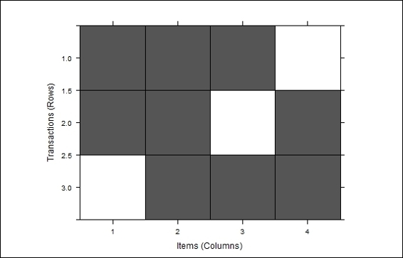
Visual inspection of transactions
6. To visually show the frequency/support bar plot, one can use itemFrequenctPlot:
7. > itemFrequencyPlot (trans)
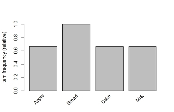
Item frequency bar plot of transactions
How it works...
As the transaction data is the base for mining associations and frequent patterns, we have to learn how to display the associations to gain insights and determine how associations are built. The arules package provides various methods to inspect transactions. First, we use the LIST function to obtain the list representation of the transaction data. We can then use the summary function to obtain information, such as basic descriptions, most frequent items, and the transaction length distribution.
Next, we use the inspect function to display the transactions. Besides displaying all transactions, one can first filter the transactions by size and then display the associations by using the inspect function. Furthermore, we can use the image function to visually inspect the transactions. Finally, we illustrate how to use the frequency/support bar plot to display the relative item frequency of each item.
See also
· Besides using itemFrequencyPlot to show the frequency/bar plot, you can use the itemFrequency function to show the support distribution. For more details, please use the help function to view the following document:
· > help(itemFrequency)
Mining associations with the Apriori rule
Association mining is a technique that can discover interesting relationships hidden in transaction datasets. This approach first finds all frequent itemsets, and generates strong association rules from frequent itemsets. Apriori is the most well-known association mining algorithm, which identifies frequent individual items first and then performs a breadth-first search strategy to extend individual items to larger itemsets until larger frequent itemsets cannot be found. In this recipe, we will introduce how to perform association analysis using the Apriori rule.
Getting ready
In this recipe, we will use the built-in transaction dataset, Groceries, to demonstrate how to perform association analysis with the Apriori algorithm in the arules package. Please make sure that the arules package is installed and loaded first.
How to do it...
Perform the following steps to analyze the association rules:
1. First, you need to load the dataset Groceries:
2. > data(Groceries)
2. You can then examine the summary of the Groceries dataset:
3. > summary(Groceries)
3. Next, you can use itemFrequencyPlot to examine the relative item frequency of itemsets:
4. > itemFrequencyPlot(Groceries, support = 0.1, cex.names=0.8, topN=5)
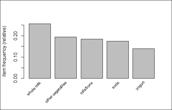
The top five item frequency bar plot of groceries transactions
4. Use apriori to discover rules with the support over 0.001 and confidence over 0.5:
5. > rules = apriori(Groceries, parameter = list(supp = 0.001, conf = 0.5, target= "rules"))
6. > summary(rules)
7. set of 5668 rules
8.
9. rule length distribution (lhs + rhs):sizes
10. 2 3 4 5 6
11. 11 1461 3211 939 46
12.
13. Min. 1st Qu. Median Mean 3rd Qu. Max.
14. 2.00 3.00 4.00 3.92 4.00 6.00
15.
16.summary of quality measures:
17. support confidence lift
18. Min. :0.001017 Min. :0.5000 Min. : 1.957
19. 1st Qu.:0.001118 1st Qu.:0.5455 1st Qu.: 2.464
20. Median :0.001322 Median :0.6000 Median : 2.899
21. Mean :0.001668 Mean :0.6250 Mean : 3.262
22. 3rd Qu.:0.001729 3rd Qu.:0.6842 3rd Qu.: 3.691
23. Max. :0.022267 Max. :1.0000 Max. :18.996
24.
25.mining info:
26. data ntransactions support confidence
27. Groceries 9835 0.001 0.5
5. We can then inspect the first few rules:
6. > inspect(head(rules))
7. lhs rhs support confidence lift
8. 1 {honey} => {whole milk} 0.001118454 0.7333333 2.870009
9. 2 {tidbits} => {rolls/buns} 0.001220132 0.5217391 2.836542
10.3 {cocoa drinks} => {whole milk} 0.001321810 0.5909091 2.312611
11.4 {pudding powder} => {whole milk} 0.001321810 0.5652174 2.212062
12.5 {cooking chocolate} => {whole milk} 0.001321810 0.5200000 2.035097
13.6 {cereals} => {whole milk} 0.003660397 0.6428571 2.515917
6. You can sort rules by confidence and inspect the first few rules:
7. > rules=sort(rules, by="confidence", decreasing=TRUE)
8. > inspect(head(rules))
9. lhs rhs support confidence lift
10.1 {rice,
11. sugar} => {whole milk} 0.001220132 1 3.913649
12.2 {canned fish,
13. hygiene articles} => {whole milk} 0.001118454 1 3.913649
14.3 {root vegetables,
15. butter,
16. rice} => {whole milk} 0.001016777 1 3.913649
17.4 {root vegetables,
18. whipped/sour cream,
19. flour} => {whole milk} 0.001728521 1 3.913649
20.5 {butter,
21. soft cheese,
22. domestic eggs} => {whole milk} 0.001016777 1 3.913649
23.6 {citrus fruit,
24. root vegetables,
25. soft cheese} => {other vegetables} 0.001016777 1 5.168156
How it works...
The purpose of association mining is to discover associations among items from the transactional database. Typically, the process of association mining proceeds by finding itemsets that have the support greater than the minimum support. Next, the process uses the frequent itemsets to generate strong rules (for example, milk => bread; a customer who buys milk is likely to buy bread) that have the confidence greater than minimum the confidence. By definition, an association rule can be expressed in the form of X=>Y, where X and Y are disjointed itemsets. We can measure the strength of associations between two terms: support and confidence. Support shows how much of the percentage of a rule is applicable within a dataset, while confidence indicates the probability of both X and Y appearing in the same transaction:
· Support = ![]()
· Confidence = 
Here, ![]() refers to the frequency of a particular itemset; N denotes the populations.
refers to the frequency of a particular itemset; N denotes the populations.
As support and confidence are metrics for the strength rule only, you might still obtain many redundant rules with a high support and confidence. Therefore, we can use the third measure, lift, to evaluate the quality (ranking) of the rule. By definition, lift indicates the strength of a rule over the random co-occurrence of X and Y, so we can formulate lift in the following form:
Lift = 
Apriori is the best known algorithm for mining associations, which performs a level-wise, breadth-first algorithm to count the candidate itemsets. The process of Apriori starts by finding frequent itemsets (a set of items that have minimum support) level-wisely. For example, the process starts with finding frequent 1-itemsets. Then, the process continues by using frequent 1-itemsets to find frequent 2-itemsets. The process iteratively discovers new frequent k+1-itemsets from frequent k-itemsets until no frequent itemsets are found.
Finally, the process utilizes frequent itemsets to generate association rules:
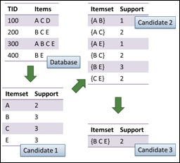
An illustration of Apriori algorithm (Where support = 2)
In this recipe, we use the Apriori algorithm to find association rules within transactions. We use the built-in Groceries dataset, which contains one month of real-world point-of-sale transaction data from a typical grocery outlet. We then use the summary function to obtain the summary statistics of the Groceries dataset. The summary statistics shows that the dataset contains 9,835 transactions, which are categorized into 169 categories. In addition to this, the summary shows information, such as most frequent items, itemset distribution, and example extended item information within the dataset. We can then use itemFrequencyPlot to visualize the five most frequent items with support over 0.1.
Next, we apply the Apriori algorithm to search for rules with support over 0.001 and confidence over 0.5. We then use the summary function to inspect detailed information on the generated rules. From the output summary, we find the Apriori algorithm generates 5,668 rules with support over 0.001 and confidence over 0.5. Further, we can find the rule length distribution, summary of quality measures, and mining information. In the summary of the quality measurement, we find descriptive statistics of three measurements, which are support, confidence, and lift. Support is the proportion of transactions containing a certain itemset. Confidence is the correctness percentage of the rule. Lift is the response target association rule divided by the average response.
To explore some generated rules, we can use the inspect function to view the first six rules of the 5,668 generated rules. Lastly, we can sort rules by confidence and list rules with the most confidence. Therefore, we find that rich sugar associated to whole milk is the most confident rule with the support equal to 0.001220132, confidence equal to 1, and lift equal to 3.913649.
See also
For those interested in the research results using the Groceries dataset, and how the support, confidence, and lift measurement are defined, you can refer to the following papers:
· Michael Hahsler, Kurt Hornik, and Thomas Reutterer (2006) Implications of probabilistic data modeling for mining association rules. In M. Spiliopoulou, R. Kruse, C. Borgelt, A
· Nuernberger, and W. Gaul, editors, From Data and Information Analysis to Knowledge Engineering, Studies in Classification, Data Analysis, and Knowledge Organization, pages 598–605. Springer-Verlag
Also, in addition to using the summary and inspect functions to inspect association rules, you can use interestMeasure to obtain additional interest measures:
> head(interestMeasure(rules, c("support", "chiSquare", "confidence", "conviction","cosine", "coverage", "leverage", "lift","oddsRatio"), Groceries))
Pruning redundant rules
Among the generated rules, we sometimes find repeated or redundant rules (for example, one rule is the super rule or subset of another rule). In this recipe, we will show you how to prune (or remove) repeated or redundant rules.
Getting ready
In this recipe, you have to complete the previous recipe by generating rules and have it stored in the variable rules.
How to do it...
Perform the following steps to prune redundant rules:
1. First, follow these steps to find redundant rules:
2. > rules.sorted = sort(rules, by="lift")
3. > subset.matrix = is.subset(rules.sorted, rules.sorted)
4. > subset.matrix[lower.tri(subset.matrix, diag=T)] = NA
5. > redundant = colSums(subset.matrix, na.rm=T) >= 1
2. You can then remove redundant rules:
3. > rules.pruned = rules.sorted[!redundant]
4. > inspect(head(rules.pruned))
5. lhs rhs support confidence lift
6. 1 {Instant food products,
7. soda} => {hamburger meat} 0.001220132 0.6315789 18.99565
8. 2 {soda,
9. popcorn} => {salty snack} 0.001220132 0.6315789 16.69779
10.3 {flour,
11. baking powder} => {sugar} 0.001016777 0.5555556 16.40807
12.4 {ham,
13. processed cheese} => {white bread} 0.001931876 0.6333333 15.04549
14.5 {whole milk,
15. Instant food products} => {hamburger meat} 0.001525165 0.5000000 15.03823
16.6 {other vegetables,
17. curd,
18. yogurt,
19. whipped/sour cream} => {cream cheese } 0.001016777 0.5882353 14.83409
How it works...
The two main constraints of association mining are to choose between the support and confidence. For example, if you use a high support threshold, you might remove rare item rules without considering whether these rules have a high confidence value. On the other hand, if you choose to use a low support threshold, the association mining can produce huge sets of redundant association rules, which make these rules difficult to utilize and analyze. Therefore, we need to prune redundant rules so we can discover meaningful information from these generated rules.
In this recipe, we demonstrate how to prune redundant rules. First, we search for redundant rules. We sort the rules by a lift measure, and then find subsets of the sorted rules using the is.subset function, which will generate an itemMatrix object. We can then set the lower triangle of the matrix to NA. Lastly, we compute colSums of the generated matrix, of which colSums >=1 indicates that the specific rule is redundant.
After we have found the redundant rules, we can prune these rules from the sorted rules. Lastly, we can examine the pruned rules using the inspect function.
See also
· In order to find subsets or supersets of rules, you can use the is.superset and is.subset functions on the association rules. These two methods may generate an itemMatrix object to show which rule is the superset or subset of other rules. You can refer to the help function for more information:
· > help(is.superset)
· > help(is.subset)
Visualizing association rules
Besides listing rules as text, you can visualize association rules, making it easier to find the relationship between itemsets. In the following recipe, we will introduce how to use the aruleViz package to visualize the association rules.
Getting ready
In this recipe, we will continue using the Groceries dataset. You need to have completed the previous recipe by generating the pruned rule rules.pruned.
How to do it...
Perform the following steps to visualize the association rule:
1. First, you need to install and load the package arulesViz:
2. > install.packages("arulesViz")
3. > library(arulesViz)
2. You can then make a scatter plot from the pruned rules:
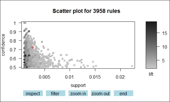
3. > plot(rules.pruned)
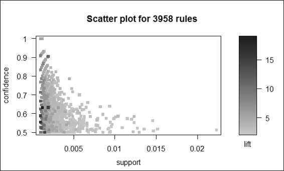
The scatter plot of pruned association rules
3. Additionally, to prevent overplotting, you can add jitter to the scatter plot:
4. > plot(rules.pruned, shading="order", control=list(jitter=6))
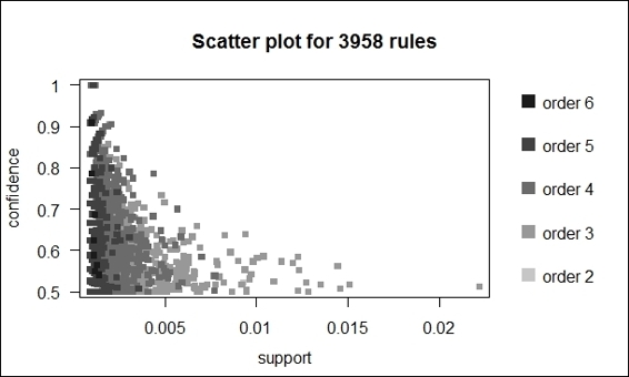
The scatter plot of pruned association rules with jitters
4. We then produce new rules with soda on the left-hand side using the Apriori algorithm:
5. > soda_rule=apriori(data=Groceries, parameter=list(supp=0.001,conf = 0.1, minlen=2), appearance = list(default="rhs",lhs="soda"))
5. Next, you can plot soda_rule in a graph plot:
6. > plot(sort(soda_rule, by="lift"), method="graph", control=list(type="items"))
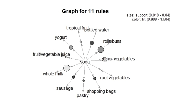
Graph plot of association rules
6. Also, the association rules can be visualized in a balloon plot:
7. > plot(soda_rule, method="grouped")
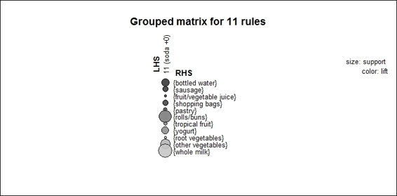
Balloon plot of association rules
How it works...
Besides presenting association rules as text, one can use arulesViz to visualize association rules. The arulesViz is an arules extension package, which provides many visualization techniques to explore association rules. To start using arulesViz, first install and load the package arulesViz. We then use the pruned rules generated in the previous recipe to make a scatter plot. As per the figure in step 2, we find the rules are shown as points within the scatter plot, with the x-axis in support and y-axis in confidence. The shade of color shows the lift of the rule; the darker the shade, the higher the lift. Next, in order to prevent overplotting points, we can include the jitter as an argument in the control list. The plot with the jitter added is provided in the figure in step 3.
In addition to plotting the rules in a scatter plot, arulesViz enables you to plot rules in a graph and grouped matrix. Instead of printing all the rules on a single plot, we choose to produce new rules with soda on the left-hand side. We then sort the rules by using the lift and visualize the rules in the graph in the figure in step 4. From the graph, every itemset is presented in a vertex and their relationship is presented in an edge. The figure (step 4) shows it is clear that the rule with soda on the left-handside to whole milk on the right-handside has the maximum support, for the size of the node is greatest. Also, the rule shows that soda on the left-hand side to bottled water on the right-hand side has the maximum lift as the shade of color in the circle is the darkest. We can then use the same data with soda on the left-handside to generate a grouped matrix, which is a balloon plot shown in the figure in step 5, with the left-handside rule as column labels and the right-handside as row labels. Similar to the graph plot in the figure in step 4, the size of the balloon in the figure in step 5 shows the support of the rule, and the color of the balloon shows the lift of the rule.
See also
· In this recipe, we introduced three visualization methods to plot association rules. However, arulesViz also provides features to plot parallel coordinate plots, double-decker plots, mosaic plots, and other related charts. For those who are interested in how these plots work, you may refer to: Hahsler, M., and Chelluboina, S. (2011). Visualizing association rules: Introduction to the R-extension package arulesViz. R project module.
· In addition to generating a static plot, you can generate an interactive plot by setting interactive equal to TRUE through the following steps:
· > plot(rules.pruned,interactive=TRUE)
The interactive scatter plots
Mining frequent itemsets with Eclat
In addition to the Apriori algorithm, you can use the Eclat algorithm to generate frequent itemsets. As the Apriori algorithm performs a breadth-first search to scan the complete database, the support counting is rather time consuming. Alternatively, if the database fits into the memory, you can use the Eclat algorithm, which performs a depth-first search to count the supports. The Eclat algorithm, therefore, performs quicker than the Apriori algorithm. In this recipe, we introduce how to use the Eclat algorithm to generate frequent itemsets.
Getting ready
In this recipe, we will continue using the dataset Groceries as our input data source.
How to do it...
Perform the following steps to generate a frequent itemset using the Eclat algorithm:
1. Similar to the Apriori method, we can use the eclat function to generate the frequent itemset:
2. > frequentsets=eclat(Groceries,parameter=list(support=0.05,maxlen=10))
2. We can then obtain the summary information from the generated frequent itemset:
3. > summary(frequentsets)
4. set of 31 itemsets
5.
6. most frequent items:
7. whole milk other vegetables yogurt
8. 4 2 2
9. rolls/buns frankfurter (Other)
10. 2 1 23
11.
12.element (itemset/transaction) length distribution:sizes
13. 1 2
14.28 3
15.
16. Min. 1st Qu. Median Mean 3rd Qu. Max.
17. 1.000 1.000 1.000 1.097 1.000 2.000
18.
19.summary of quality measures:
20. support
21. Min. :0.05236
22. 1st Qu.:0.05831
23. Median :0.07565
24. Mean :0.09212
25. 3rd Qu.:0.10173
26. Max. :0.25552
27.
28.includes transaction ID lists: FALSE
29.
30.mining info:
31. data ntransactions support
32. Groceries 9835 0.05
3. Lastly, we can examine the top ten support frequent itemsets:
4. > inspect(sort(frequentsets,by="support")[1:10])
5. items support
6. 1 {whole milk} 0.25551601
7. 2 {other vegetables} 0.19349263
8. 3 {rolls/buns} 0.18393493
9. 4 {soda} 0.17437722
10.5 {yogurt} 0.13950178
11.6 {bottled water} 0.11052364
12.7 {root vegetables} 0.10899847
13.8 {tropical fruit} 0.10493137
14.9 {shopping bags} 0.09852567
15.10 {sausage} 0.09395018
How it works...
In this recipe, we introduce another algorithm, Eclat, to perform frequent itemset generation. Though Apriori is a straightforward and easy to understand association mining method, the algorithm has the disadvantage of generating huge candidate sets and performs inefficiently in support counting, for it takes multiple scans of databases. In contrast to Apriori, Eclat uses equivalence classes, depth-first searches, and set intersections, which greatly improves the speed in support counting.
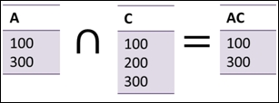
In Apriori, the algorithm uses a horizontal data layout to store transactions. On the other hand, Eclat uses a vertical data layout to store a list of transaction IDs (tid) for each item. Then, Eclat determines the support of any k+1-itemset by intersecting tid-lists of two k-itemsets. Lastly, Eclat utilizes frequent itemsets to generate association rules:
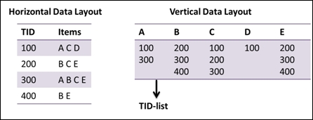
An illustration of Eclat algorithm
Similar to the recipe using the Apriori algorithm, we can use the eclat function to generate a frequent itemset with a given support (assume support = 2 in this case) and maximum length.
Generating frequent itemset
We can then use the summary function to obtain summary statistics, which include: most frequent items, itemset length distributions, summary of quality measures, and mining information. Finally, we can sort frequent itemsets by the support and inspect the top ten support frequent itemsets.
See also
· Besides Apriori and Eclat, another popular association mining algorithm is FP-Growth. Similar to Eclat, this takes a depth-first search to count supports. However, there is no existing R package that you can download from CRAN that contains this algorithm. However, if you are interested in knowing how to apply the FP-growth algorithm in your transaction dataset, you can refer to Christian Borgelt's page at http://www.borgelt.net/fpgrowth.html for more information.
Creating transactions with temporal information
In addition to mining interesting associations within the transaction database, we can mine interesting sequential patterns using transactions with temporal information. In the following recipe, we demonstrate how to create transactions with temporal information.
Getting ready
In this recipe, we will generate transactions with temporal information. We can use the generated transactions as the input source for frequent sequential pattern mining.
How to do it...
Perform the following steps to create transactions with temporal information:
1. First, you need to install and load the package arulesSequences:
2. > install.packages("arulesSequences")
3. > library(arulesSequences)
2. You can first create a list with purchasing records:
3. > tmp_data=list(c("A"),
4. + c("A","B","C"),
5. + c("A","C"),
6. + c("D"),
7. + c("C","F"),
8. + c("A","D"),
9. + c("C"),
10.+ c("B","C"),
11.+ c("A","E"),
12.+ c("E","F"),
13.+ c("A","B"),
14.+ c("D","F"),
15.+ c("C"),
16.+ c("B"),
17.+ c("E"),
18.+ c("G"),
19.+ c("A","F"),
20.+ c("C"),
21.+ c("B"),
22.+ c("C"))
3. You can then turn the list into transactions and add temporal information:
4. >names(tmp_data) = paste("Tr",c(1:20), sep = "")
5. >trans = as(tmp_data,"transactions")
6. >transactionInfo(trans)$sequenceID=c(1,1,1,1,1,2,2,2,2,3,3,3,3,3,4,4,4,4,4,4)
7. >transactionInfo(trans)$eventID=c(10,20,30,40,50,10,20,30,40,10,20,30,40,50,10,20,30,40,50,60)
8. > trans
9. transactions in sparse format with
10. 20 transactions (rows) and
11. 7 items (columns)
4. Next, you can use the inspect function to inspect the transactions:
5. > inspect(head(trans))
6. items transactionID sequenceID eventID
7. 1 {A} Tr1 1 10
8. 2 {A,
9. B,
10. C} Tr2 1 20
11.3 {A,
12. C} Tr3 1 30
13.4 {D} Tr4 1 40
14.5 {C,
15. F} Tr5 1 50
16.6 {A,
17. D} Tr6 2 10
5. You can then obtain the summary information of the transactions with the temporal information:
6. > summary(trans)
7. transactions as itemMatrix in sparse format with
8. 20 rows (elements/itemsets/transactions) and
9. 7 columns (items) and a density of 0.2214286
10.
11.most frequent items:
12. C A B F D (Other)
13. 8 7 5 4 3 4
14.
15.element (itemset/transaction) length distribution:
16.sizes
17. 1 2 3
18.10 9 1
19.
20. Min. 1st Qu. Median Mean 3rd Qu. Max.
21. 1.00 1.00 1.50 1.55 2.00 3.00
22.
23.includes extended item information - examples:
24. labels
25.1 A
26.2 B
27.3 C
28.
29.includes extended transaction information - examples:
30. transactionID sequenceID eventID
31.1 Tr1 1 10
32.2 Tr2 1 20
33.3 Tr3 1 30
6. You can also read the transaction data in a basket format:
7. > zaki=read_baskets(con = system.file("misc", "zaki.txt", package = "arulesSequences"), info = c("sequenceID","eventID","SIZE"))
8. > as(zaki, "data.frame")
9. transactionID.sequenceID transactionID.eventID transactionID.SIZE items
10.1 1 10 2 {C,D}
11.2 1 15 3 {A,B,C}
12.3 1 20 3 {A,B,F}
13.4 1 25 4 {A,C,D,F}
14.5 2 15 3 {A,B,F}
15.6 2 20 1 {E}
16.7 3 10 3 {A,B,F}
17.8 4 10 3 {D,G,H}
18.9 4 20 2 {B,F}
19.10 4 25 3 {A,G,H}
How it works...
Before mining frequent sequential patterns, you are required to create transactions with the temporal information. In this recipe, we introduce two methods to obtain transactions with temporal information. In the first method, we create a list of transactions, and assign a transaction ID for each transaction. We use the as function to transform the list data into a transaction dataset. We then add eventID and sequenceID as temporal information; sequenceID is the sequence that the event belongs to, and eventID indicates when the event occurred. After generating transactions with temporal information, one can use this dataset for frequent sequential pattern mining.
In addition to creating your own transactions with temporal information, if you already have data stored in a text file, you can use the read_basket function from arulesSequences to read the transaction data into the basket format. We can also read the transaction dataset for further frequent sequential pattern mining.
See also
· The arulesSequences function provides two additional data structures, sequences and timedsequences, to present pure sequence data and sequence data with the time information. For those who are interested in these two collections, please use the help function to view the following documents:
· > help("sequences-class")
· > help("timedsequences-class")
Mining frequent sequential patterns with cSPADE
In contrast to association mining, which only discovers relationships between itemsets, we may be interested in exploring patterns shared among transactions where a set of itemsets occurs sequentially.
One of the most famous frequent sequential pattern mining algorithms is the Sequential PAttern Discovery using Equivalence classes (SPADE) algorithm, which employs the characteristics of a vertical database to perform an intersection on an ID list with an efficient lattice search and allows us to place constraints on mined sequences. In this recipe, we will demonstrate how to use cSPADE to mine frequent sequential patterns.
Getting ready
In this recipe, you have to complete the previous recipes by generating transactions with the temporal information and have it stored in the variable trans.
How to do it...
Perform the following steps to mine the frequent sequential patterns:
1. First, you can use the cspade function to generate frequent sequential patterns:
2. > s_result=cspade(trans,parameter = list(support = 0.75),control = list(verbose = TRUE))
2. You can then examine the summary of the frequent sequential patterns:
3. > summary(s_result)
4. set of 14 sequences with
5.
6. most frequent items:
7. C A B D E (Other)
8. 8 5 5 2 1 1
9.
10.most frequent elements:
11. {C} {A} {B} {D} {E} (Other)
12. 8 5 5 2 1 1
13.
14.element (sequence) size distribution:
15.sizes
16.1 2 3
17.6 6 2
18.
19.sequence length distribution:
20.lengths
21.1 2 3
22.6 6 2
23.
24.summary of quality measures:
25. support
26. Min. :0.7500
27. 1st Qu.:0.7500
28. Median :0.7500
29. Mean :0.8393
30. 3rd Qu.:1.0000
31. Max. :1.0000
32.
33.includes transaction ID lists: FALSE
34.
35.mining info:
36. data ntransactions nsequences support
37. trans 20 4 0.75
3. Transform a generated sequence format data back to the data frame:
4. > as(s_result, "data.frame")
5. sequence support
6. 1 <{A}> 1.00
7. 2 <{B}> 1.00
8. 3 <{C}> 1.00
9. 4 <{D}> 0.75
10.5 <{E}> 0.75
11.6 <{F}> 0.75
12.7 <{A},{C}> 1.00
13.8 <{B},{C}> 0.75
14.9 <{C},{C}> 0.75
15.10 <{D},{C}> 0.75
16.11 <{A},{C},{C}> 0.75
17.12 <{A},{B}> 1.00
18.13 <{C},{B}> 0.75
19.14 <{A},{C},{B}> 0.75
How it works...
The object of sequential pattern mining is to discover sequential relationships or patterns in transactions. You can use the pattern mining result to predict future events, or recommend items to users.
One popular method of sequential pattern mining is SPADE. SPADE uses a vertical data layout to store a list of IDs. In these, each input sequence in the database is called SID, and each event in a given input sequence is called EID. The process of SPADE is performed by generating patterns level-wisely by an Apriori candidate generation. In detail, SPADE generates subsequent n-sequences from joining (n-1)-sequences from the intersection of ID lists. If the number of sequences is greater than the minimum support (minsup), we can consider the sequence to be frequent enough. The algorithm stops until the process cannot find more frequent sequences:
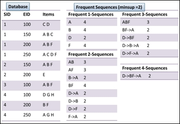
An illustration of SPADE algorithm
In this recipe, we illustrate how to use a frequent sequential pattern mining algorithm, cSPADE, to mine frequent sequential patterns. First, as we have transactions with temporal information loaded in the variable trans, we can use the cspade function with the support over 0.75 to generate frequent sequential patterns in the sequences format. We can then obtain summary information, such as most frequent items, sequence size distributions, a summary of quality measures, and mining information. Lastly, we can transform the generated sequence information back to the data frame format, so we can examine the sequence and support of frequent sequential patterns with the support over 0.75.
See also
· If you are interested in the concept and design of the SPADE algorithm, you can refer to the original published paper: M. J. Zaki. (2001). SPADE: An Efficient Algorithm for Mining Frequent Sequences. Machine Learning Journal, 42, 31–60.
All materials on the site are licensed Creative Commons Attribution-Sharealike 3.0 Unported CC BY-SA 3.0 & GNU Free Documentation License (GFDL)
If you are the copyright holder of any material contained on our site and intend to remove it, please contact our site administrator for approval.
© 2016-2026 All site design rights belong to S.Y.A.