Machine Learning with R Cookbook (2015)
Chapter 4. Understanding Regression Analysis
In this chapter, we will cover the following recipes:
· Fitting a linear regression model with lm
· Summarizing linear model fits
· Using linear regression to predict unknown values
· Generating a diagnostic plot of a fitted model
· Fitting a polynomial regression model with lm
· Fitting a robust linear regression model with rlm
· Studying a case of linear regression on SLID data
· Applying the Gaussian model for generalized linear regression
· Applying the Poisson model for generalized linear regression
· Applying the Binomial model for generalized linear regression
· Fitting a generalized additive model to data
· Visualizing a generalized additive model
· Diagnosing a generalized additive model
Introduction
Regression is a supervised learning method, which is employed to model and analyze the relationship between a dependent (response) variable and one or more independent (predictor) variables. One can use regression to build a prediction model, which can first be used to find the best fitted model with minimum squared errors of the fitted values. The fitted model can then be further applied to data for continuous value predictions.
There are many types of regression. If there is only one predictor variable, and the relationship between the response variable and independent variable is linear, we can apply a linear model. However, if there is more than one predictor variable, a multiple linear regression method should be used. When the relationship is nonlinear, one can use a nonlinear model to model the relationship between the predictor and response variables.
In this chapter, we introduce how to fit a linear model into data with the lm function. Next, for distribution in other than the normal Gaussian model (for example, Poisson or Binomial), we use the glm function with an appropriate link function correspondent to the data distribution. Finally, we cover how to fit a generalized additive model into data using the gam function.
Fitting a linear regression model with lm
The simplest model in regression is linear regression, which is best used when there is only one predictor variable, and the relationship between the response variable and the independent variable is linear. In R, we can fit a linear model to data with the lm function.
Getting ready
We need to prepare data with one predictor and response variable, and with a linear relationship between the two variables.
How to do it...
Perform the following steps to perform linear regression with lm:
1. You should install the car package and load its library:
2. > install.packages("car")
3. > library(car)
2. From the package, you can load the Quartet dataset:
3. > data(Quartet)
3. You can use the str function to display the structure of the Quartet dataset:
4. > str(Quartet)
5. 'data.frame': 11 obs. of 6 variables:
6. $ x : int 10 8 13 9 11 14 6 4 12 7 ...
7. $ y1: num 8.04 6.95 7.58 8.81 8.33 ...
8. $ y2: num 9.14 8.14 8.74 8.77 9.26 8.1 6.13 3.1 9.13 7.26 ...
9. $ y3: num 7.46 6.77 12.74 7.11 7.81 ...
10. $ x4: int 8 8 8 8 8 8 8 19 8 8 ...
11. $ y4: num 6.58 5.76 7.71 8.84 8.47 7.04 5.25 12.5 5.56 7.91 ...
4. Draw a scatter plot of the x and y variables with plot, and append a fitted line through the lm and abline function:
5. > plot(Quartet$x, Quartet$y1)
6. > lmfit = lm(y1~x, Quartet)
7. > abline(lmfit, col="red")
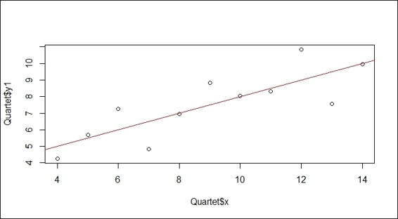
A simple regression plot fitted by lm
5. To view the fit model, execute the following:
6. > lmfit
7.
8. Call:
9. lm(formula = y1 ~ x, data = Quartet)
10.
11.Coefficients:
12.(Intercept) x
13. 3.0001 0.5001
How it works...
The regression model has the response ~ terms form, where response is the response vector, and terms is a series of terms that specifies a predictor. We can illustrate a simple regression model in the formula y=α+βx, where α is the intercept while the slope, β, describes the change in y when x changes. By using the least squares method, we can estimate 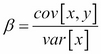 and
and ![]() (where
(where ![]() indicates the mean value of y and
indicates the mean value of y and ![]() denotes the mean value of x).
denotes the mean value of x).
To perform linear regression, we first prepare the data that has a linear relationship between the predictor variable and response variable. In this example, we load Anscombe's quartet dataset from the package car. Within the dataset, the x and y1 variables have a linear relationship, and we prepare a scatter plot of these variables. To generate the regression line, we use the lm function to generate a model of the two variables. Further, we use abline to plot a regression line on the plot. As per the previous screenshot, the regression line illustrates the linear relationship of x and y1 variables. We can see that the coefficient of the fitted model shows the intercept equals 3.0001 and coefficient equals 0.5001. As a result, we can use the intercept and coefficient to infer the response value. For example, we can infer the response value when x at 3 is equal to 4.5103 (3 * 0.5001 + 3.0001).
There's more...
Besides the lm function, you can also use the lsfit function to perform simple linear regression. For example:
> plot(Quartet$x, Quartet$y1)
> lmfit2 = lsfit(Quartet$x,Quartet$y1)
> abline(lmfit2, col="red")
A simple regression fitted by the lsfit function.
Summarizing linear model fits
The summary function can be used to obtain the formatted coefficient, standard errors, degree of freedom, and other summarized information of a fitted model. This recipe introduces how to obtain overall information on a model through the use of the summary function.
Getting ready
You need to have completed the previous recipe by computing the linear model of the x and y1 variables from the quartet, and have the fitted model assigned to the lmfit variable.
How to do it...
Perform the following step to summarize linear model fits:
1. Compute a detailed summary of the fitted model:
2. > summary(lmfit)
3.
4. Call:
5. lm(formula = y1 ~ x)
6.
7. Residuals:
8. Min 1Q Median 3Q Max
9. -1.92127 -0.45577 -0.04136 0.70941 1.83882
10.
11.Coefficients:
12. Estimate Std. Error t value Pr(>|t|)
13.(Intercept) 3.0001 1.1247 2.667 0.02573 *
14.Quartet$x 0.5001 0.1179 4.241 0.00217 **
15.---
16.Signif. codes: 0 '***' 0.001 '**' 0.01 '*' 0.05 '.' 0.1 ' ' 1
17.
18.Residual standard error: 1.237 on 9 degrees of freedom
19.Multiple R-squared: 0.6665, Adjusted R-squared: 0.6295
20.F-statistic: 17.99 on 1 and 9 DF, p-value: 0.00217
How it works...
The summary function is a generic function used to produce summary statistics. In this case, it computes and returns a list of the summary statistics of the fitted linear model. Here, it will output information such as residuals, coefficient standard error R-squared, f-statistic, and a degree of freedom. In the Call section, the function called to generate the fitted model is displayed. In the Residuals section, it provides a quick summary (min, 1Q, median, 3Q, max) of the distribution.
In the Coefficients section, each coefficient is a Gaussian random variable. Within this section, Estimate represents the mean distribution of the variable; Std.Error displays the standard error of the variable; the t value is Estimatedivided by Std.Error and the p value indicates the probability of getting a value larger than the t value. In this sample, the p value of both intercepts (0.002573) and x (0.00217) have a 95 percent level of confidence.
Residual standard error outputs the standard deviation of residuals, while the degree of freedom indicates the differences between the observation in training samples and the number used in the model. Multiple R-squared is obtained by dividing the sum of squares. One can use R-squared to measure how close the data is to fit into the regression line. Mostly, the higher the R-squared, the better the model fits your data. However, it does not necessarily indicate whether the regression model is adequate. This means you might get a good model with a low R-squared or you can have a bad model with a high R-squared. Since multiple R-squared ignore a degree of freedom, the calculated score is biased. To make the calculation fair, an adjusted R-squared (0.6295) uses an unbiased estimate, and will be slightly less than multiple R-squared (0.6665). F-statistic is retrieved by performing an f-test on the model. A pvalue equal to 0.00217 (< 0.05) rejects the null hypothesis (no linear correlation between variables) and indicates that the observed F is greater than the critical F value. In other words, the result shows that there is a significant positive linear correlation between the variables.
See also
· For more information on the parameters used for obtaining a summary of the fitted model, you can use the help function or ? to view the help page:
· > ?summary.lm
· Alternatively, you can use the following functions to display the properties of the model:
· > coefficients(lmfit) # Extract model coefficients
· > confint(lmfit, level=0.95) # Computes confidence intervals for model parameters.
· > fitted(lmfit) # Extract model fitted values
· > residuals(lmfit) # Extract model residuals
· > anova(lmfit) # Compute analysis of variance tables for fitted model object
· > vcov(lmfit) # Calculate variance-covariance matrix for a fitted model object
· > influence(lmfit) # Diagnose quality of regression fits
Using linear regression to predict unknown values
With a fitted regression model, we can apply the model to predict unknown values. For regression models, we can express the precision of prediction with a prediction interval and a confidence interval. In the following recipe, we introduce how to predict unknown values under these two measurements.
Getting ready
You need to have completed the previous recipe by computing the linear model of the x and y1 variables from the quartet dataset.
How to do it...
Perform the following steps to predict values with linear regression:
1. Fit a linear model with the x and y1 variables:
2. > lmfit = lm(y1~x, Quartet)
2. Assign values to be predicted into newdata:
3. > newdata = data.frame(x = c(3,6,15))
3. Compute the prediction result using the confidence interval with level set as 0.95:
4. > predict(lmfit, newdata, interval="confidence", level=0.95)
5. fit lwr upr
6. 1 4.500364 2.691375 6.309352
7. 2 6.000636 4.838027 7.163245
8. 3 10.501455 8.692466 12.310443
4. Compute the prediction result using this prediction interval:
5. > predict(lmfit, newdata, interval="predict")
6. fit lwr upr
7. 1 4.500364 1.169022 7.831705
8. 2 6.000636 2.971271 9.030002
9. 3 10.501455 7.170113 13.832796
How it works...
We first build a linear fitted model with x and y1 variables. Next, we assign values to be predicted into a data frame, newdata. It is important to note that the generated model is in the form of y1 ~ x.
Next, we compute the prediction result using a confidence interval by specifying confidence in the argument interval. From the output of row 1, we get fitted y1 of the x=3 input, which equals to 4.500364, and a 95 percent confidence interval (set 0.95 in the level argument) of the y1 mean for x=3 is between 2.691375 and 6.309352. In addition to this, row 2 and 3 give the prediction result of y1 with an input of x=6 and x=15.
Next, we compute the prediction result using a prediction interval by specifying prediction in the argument interval. From the output of row 1, we can see fitted y1 of the x=3 input equals to 4.500364, and a 95 percent prediction interval of y1 for x=3 is between 1.169022 and 7.831705. Row 2 and 3 output the prediction result of y1 with an input of x=6 and x=15.
See also
· For those who are interested in the differences between prediction intervals and confidence intervals, you can refer to the Wikipedia entry contrast with confidence intervals at http://en.wikipedia.org/wiki/Prediction_interval#Contrast_with_confidence_intervals.
Generating a diagnostic plot of a fitted model
Diagnostics are methods to evaluate assumptions of the regression, which can be used to determine whether a fitted model adequately represents the data. In the following recipe, we introduce how to diagnose a regression model through the use of a diagnostic plot.
Getting ready
You need to have completed the previous recipe by computing a linear model of the x and y1 variables from the quartet, and have the model assigned to the lmfit variable.
How to do it...
Perform the following step to generate a diagnostic plot of the fitted model:
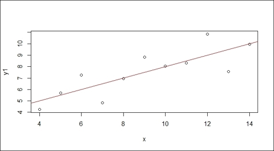
1. Plot the diagnostic plot of the regression model:
2. > par(mfrow=c(2,2))
3. > plot(lmfit)
Diagnostic plots of the regression model
How it works...
The plot function generates four diagnostic plots of a regression model:
· The upper-left plot shows residuals versus fitted values. Within the plot, residuals represent the vertical distance from a point to the regression line. If all points fall exactly on the regression line, all residuals will fall exactly on the dotted gray line. The red line within the plot is a smooth curve with regard to residuals, and if all the dots fall exactly on the regression line, the position of the red line should exactly match the dotted gray line.
· The upper-right shows the normal of residuals. This plot verifies the assumption that residuals were normally distributed. Thus, if the residuals were normally distributed, they should lie exactly on the gray dash line.
· The Scale-Location plot on the bottom-left is used to measure the square root of the standardized residuals against the fitted value. Therefore, if all dots lie on the regression line, the value of y should be close to zero. Since it is assumed that the variance of residuals does not change the distribution substantially, if the assumption is correct, the red line should be relatively flat.
· The bottom-right plot shows standardized residuals versus leverage. The leverage is a measurement of how each data point influences the regression. It is a measurement of the distance from the centroid of regression and level of isolation (measured by whether it has neighbors). Also, you can find the contour of Cook's distance, which is affected by high leverage and large residuals. You can use this to measure how regression would change if a single point is deleted. The red line is smooth with regard to standardized residuals. For a perfect fit regression, the red line should be close to the dashed line with no points over 0.5 in Cook's distance.
There's more...
To see more of the diagnostic plot function, you can use the help function to access further information:
> ?plot.lm
In order to discover whether there are points with large Cook's distance, one can use the cooks.distance function to compute the Cook's distance of each point, and analyze the distribution of distance through visualization:
> plot(cooks.distance(lmfit))
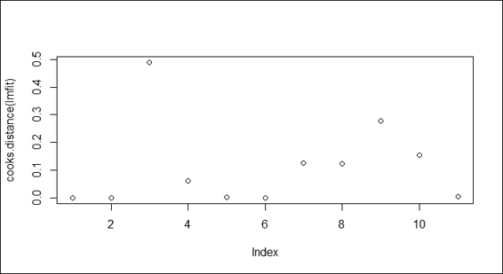
A plot of Cook's distance
In this case, where the point on index 3 shows greater Cook's distance than other points, one can investigate whether this point might be an outlier.
Fitting a polynomial regression model with lm
Some predictor variables and response variables may have a non-linear relationship, and their relationship can be modeled as an nth order polynomial. In this recipe, we introduce how to deal with polynomial regression using the lmand poly functions.
Getting ready
Prepare the dataset that includes a relationship between the predictor and response variable that can be modeled as an nth order polynomial. In this recipe, we will continue to use the Quartet dataset from the car package.
How to do it...
Perform the following steps to fit the polynomial regression model with lm:
1. First, we make a scatter plot of the x and y2 variables:
2. > plot(Quartet$x, Quartet$y2)
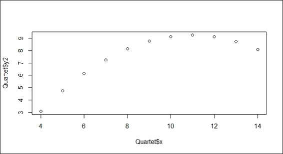
Scatter plot of variables x and y2
2. You can apply the poly function by specifying 2 in the argument:
3. > lmfit = lm(Quartet$y2~poly(Quartet$x,2))
4. > lines(sort(Quartet$x), lmfit$fit[order(Quartet$x)], col = "red")
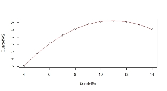
A quardratic fit example of the regression plot of variables x and y2
How it works
We can illustrate the second order polynomial regression model in formula, ![]() , where α is the intercept while β, illustrates regression coefficients.
, where α is the intercept while β, illustrates regression coefficients.
In the preceding screenshot (step 1), the scatter plot of the x and y2 variables does not fit in a linear relationship, but shows a concave downward curve (or convex upward) with the turning point at x=11. In order to model the nonlinear relationship, we apply the poly function with an argument of 2 to fit the independent x variable and the dependent y2 variable. The red line in the screenshot shows that the model perfectly fits the data.
There's more...
You can also fit a second order polynomial model with an independent variable equal to the formula of the combined first order x variable and the second order x variable:
> plot(Quartet$x, Quartet$y2)
> lmfit = lm(Quartet$y2~ I(Quartet$x)+I(Quartet$x^2))
Fitting a robust linear regression model with rlm
An outlier in the dataset will move the regression line away from the mainstream. Apart from removing it, we can apply a robust linear regression to fit datasets containing outliers. In this recipe, we introduce how to apply rlm to perform robust linear regression to datasets containing outliers.
Getting ready
Prepare the dataset that contains an outlier that may move the regression line away from the mainstream. Here, we use the Quartet dataset loaded from the previous recipe.
How to do it...
Perform the following steps to fit the robust linear regression model with rlm:
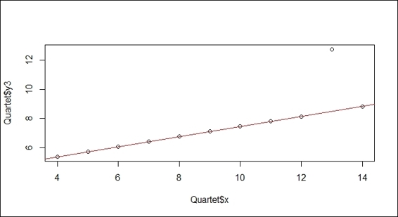
1. Generate a scatter plot of the x variable against y3:
2. > plot(Quartet$x, Quartet$y3)
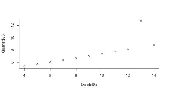
Scatter plot of variables x and y3
2. Next, you should import the MASS library first. Then, you can apply the rlm function to fit the model, and visualize the fitted line with the abline function:
3. > library(MASS)
4. > lmfit = rlm(Quartet$y3~Quartet$x)
5. > abline(lmfit, col="red")
Robust linear regression to variables x and y3
How it works
As per the preceding screenshot (step 1), you may encounter datasets that include outliers away from the mainstream. To remove the effect of an outlier, we demonstrate how to apply a robust linear regression (rlm) to fit the data. In the second screenshot (step 2), the robust regression line ignores the outlier and matches the mainstream.
There's more...
To see the effect of how an outlier can move the regression line away from the mainstream, you may replace the rlm function used in this recipe to lm, and replot the graph:
> plot(Quartet$x, Quartet$y3)
> lmfit = lm(Quartet$y3~Quartet$x)
> abline(lmfit, col="red")
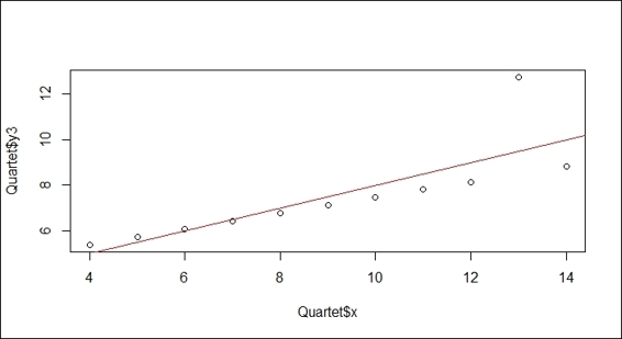
Linear regression on variables x and y3
It is obvious that outlier (x=13) moves the regression line away from the mainstream.
Studying a case of linear regression on SLID data
To summarize the contents of the previous section, we explore more complex data with linear regression. In this recipe, we demonstrate how to apply linear regression to analyze the Survey of Labor and Income Dynamics (SLID) dataset.
Getting ready
Check whether the car library is installed and loaded, as it is required to access thedataset SLID.
How to do it...
Follow these steps to perform linear regression on SLID data:
1. You can use the str function to get an overview of the data:
2. > str(SLID)
3. 'data.frame': 7425 obs. of 5 variables:
4. $ wages : num 10.6 11 NA 17.8 NA ...
5. $ education: num 15 13.2 16 14 8 16 12 14.5 15 10 ...
6. $ age : int 40 19 49 46 71 50 70 42 31 56 ...
7. $ sex : Factor w/ 2 levels "Female","Male": 2 2 2 2 2 1 1 1 2 1 ...
8. $ language : Factor w/ 3 levels "English","French",..: 1 1 3 3 1 1 1 1 1 1 ..
2. First, we visualize the variable wages against language, age, education, and sex:
3. > par(mfrow=c(2,2))
4. > plot(SLID$wages ~ SLID$language)
5. > plot(SLID$wages ~ SLID$age)
6. > plot(SLID$wages ~ SLID$education)
7. > plot(SLID$wages ~ SLID$sex)
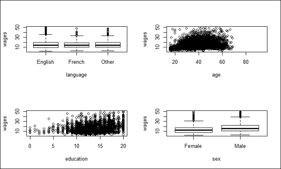
Plot of wages against multiple combinations
3. Then, we can use lm to fit the model:
4. > lmfit = lm(wages ~ ., data = SLID)
4. You can examine the summary of the fitted model through the summary function:
5. > summary(lmfit)
6.
7. Call:
8. lm(formula = wages ~ ., data = SLID)
9.
10.Residuals:
11. Min 1Q Median 3Q Max
12.-26.062 -4.347 -0.797 3.237 35.908
13.
14.Coefficients:
15. Estimate Std. Error t value Pr(>|t|)
16.(Intercept) -7.888779 0.612263 -12.885 <2e-16 ***
17.education 0.916614 0.034762 26.368 <2e-16 ***
18.age 0.255137 0.008714 29.278 <2e-16 ***
19.sexMale 3.455411 0.209195 16.518 <2e-16 ***
20.languageFrench -0.015223 0.426732 -0.036 0.972
21.languageOther 0.142605 0.325058 0.439 0.661
22.---
23.Signif. codes: 0 '***' 0.001 '**' 0.01 '*' 0.05 '.' 0.1 ' ' 1
24.
25.Residual standard error: 6.6 on 3981 degrees of freedom
26. (3438 observations deleted due to missingness)
27.Multiple R-squared: 0.2973, Adjusted R-squared: 0.2964
28.F-statistic: 336.8 on 5 and 3981 DF, p-value: < 2.2e-16
5. Drop the language attribute, and refit the model with the lm function:
6. > lmfit = lm(wages ~ age + sex + education, data = SLID)
7. > summary(lmfit)
8.
9. Call:
10.lm(formula = wages ~ age + sex + education, data = SLID)
11.
12.Residuals:
13. Min 1Q Median 3Q Max
14.-26.111 -4.328 -0.792 3.243 35.892
15.
16.Coefficients:
17. Estimate Std. Error t value Pr(>|t|)
18.(Intercept) -7.905243 0.607771 -13.01 <2e-16 ***
19.age 0.255101 0.008634 29.55 <2e-16 ***
20.sexMale 3.465251 0.208494 16.62 <2e-16 ***
21.education 0.918735 0.034514 26.62 <2e-16 ***
22.---
23.Signif. codes: 0 '***' 0.001 '**' 0.01 '*' 0.05 '.' 0.1 ' ' 1
24.
25.Residual standard error: 6.602 on 4010 degrees of freedom
26. (3411 observations deleted due to missingness)
27.Multiple R-squared: 0.2972, Adjusted R-squared: 0.2967
28.F-statistic: 565.3 on 3 and 4010 DF, p-value: < 2.2e-16
6. We can then draw a diagnostic plot of lmfit:
7. > par(mfrow=c(2,2))
8. > plot(lmfit)
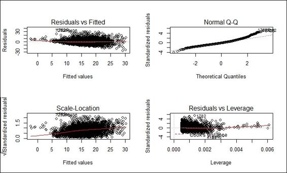
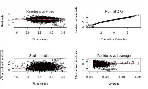
Diagnostic plot of fitted model
7. Next, we take the log of wages and replot the diagnostic plot:
8. > lmfit = lm(log(wages) ~ age + sex + education, data = SLID)
9. > plot(lmfit)
Diagnostic plot of adjusted fitted model
8. Next, you can diagnose the multi-colinearity of the regression model using the vif function:
9. > vif(lmfit)
10. age sex education
11. 1.011613 1.000834 1.012179
12.> sqrt(vif(lmfit)) > 2
13. age sex education
14. FALSE FALSE FALSE
9. Then, you can install and load the lmtest package and diagnose the heteroscedasticity of the regression model with the bptest function:
10.> install.packages("lmtest")
11.> library(lmtest)
12.> bptest(lmfit)
13.
14. studentized Breusch-Pagan test
15.
16.data: lmfit
17.BP = 29.0311, df = 3, p-value = 2.206e-06
10.Finally, you can install and load the rms package. Then, you can correct standard errors with robcov:
11.> install.packages("rms")
12.> library(rms)
13.> olsfit = ols(log(wages) ~ age + sex + education, data= SLID, x= TRUE, y= TRUE)
14.> robcov(olsfit)
15.
16.Linear Regression Model
17.
18.ols(formula = log(wages) ~ age + sex + education, data = SLID,
19. x = TRUE, y = TRUE)
20.
21.Frequencies of Missing Values Due to Each Variable
22.log(wages) age sex education
23. 3278 0 0 249
24.
25.
26. Model Likelihood Discrimination
27. Ratio Test Indexes
28.Obs 4014 LR chi2 1486.08 R2 0.309
29.sigma 0.4187 d.f. 3 R2 adj 0.309
30.d.f. 4010 Pr(> chi2) 0.0000 g 0.315
31.
32.Residuals
33.
34. Min 1Q Median 3Q Max
35.-2.36252 -0.27716 0.01428 0.28625 1.56588
36.
37. Coef S.E. t Pr(>|t|)
38.Intercept 1.1169 0.0387 28.90 <0.0001
39.age 0.0176 0.0006 30.15 <0.0001
40.sex=Male 0.2244 0.0132 16.96 <0.0001
41.education 0.0552 0.0022 24.82 <0.0001
How it works...
This recipe demonstrates how to conduct linear regression analysis on the SLID dataset. First, we load the SLID data and display its structure through the use of the str function. From the structure of the data, we know that there are four independent variables that will affect the wages of the dependent variable.
Next, we explore the relationship of each independent variable to the dependent variable, wages, through visualization; the visualization result is shown in the preceding screenshot (step 2). In the upper-left section of this screenshot, you can find the box plot of three different languages against wages; the correlation between the languages and wages is not obvious. The upper-right section of the screenshot shows that the age appears to have a positive relationship with the dependent variable, wages. In the bottom-left of the screenshot, it is shown that education also appears to have a positive relationship with wages. Finally, the box plot in the bottom-right section of the screenshot shows that the wages of males are slightly higher than females.
Next, we fit all the attributes except for wages to the model as predictor variables. By summarizing the model, it is shown that education, age, and sex show a significance (p-value < 0.05). As a result, we drop the insignificant language attribute (which has a p-value greater than 0.05) and fit the three independent variables (education, sex, and age) with regard to the dependent variable (wages) in the linear model. This accordingly raises the f-statistic from 336.8 to 565.3.
Next, we generate the diagnostic plot of the fitted model. Within the diagnostic plot, all the four plots indicate that the regression model follows the regression assumption. However, from residuals versus fitted and scale-location plot, residuals of smaller fitted values are biased toward the regression model. Since wages range over several orders of magnitude, to induce the symmetry, we apply a log transformation to wages and refit the data into a regression model. The red line of residuals versus fitted values plot and the Scale-Location plot are now closer to the gray dashed line.
Next, we would like to test whether multi-colinearity exists in the model. Multi-colinearity takes place when a predictor is highly correlated with others. If multi-colinearity exists in the model, you might see some variables have a high R-squared value but are shown as variables insignificant. To detect multi-colinearity, we can calculate the variance inflation and generalized variance inflation factors for linear and generalized linear models with the viffunction. If multi-colinearity exists, we should find predictors with the square root of variance inflation factor above 2. Then, we may remove redundant predictors or use a principal component analysis to transform predictors to a smaller set of uncorrelated components.
Finally, we would like to test whether heteroscedasticity exists in the model. Before discussing the definition of heteroscedasticity, we first have to know that in classic assumptions, the ordinary regression model assumes that the variance of the error is constant or homogeneous across observations. On the contrary, heteroscedasticity means that the variance is unequal across observations. As a result, heteroscedasticity may be biased toward the standard errors of our estimates and, therefore, mislead the testing of the hypothes. To detect and test heteroscedasticity, we can perform the Breusch-Pagan test for heteroscedasticity with the bptest function within the lmtest package. In this case, the p-value shows 2.206e-06 (<0.5), which rejects the null hypothesis of homoscedasticity (no heteroscedasticity). Here, it implies that the standard errors of the parameter estimates are incorrect. However, we can use robust standard errors to correct the standard error (do not remove the heteroscedasticity) and increase the significance of truly significant parameters with robcov from the rms package. However, since it only takes the fitted model from the rms series as an input, we have to fit the ordinary least squares model beforehand.
See also
· For more information about the SLID dataset, you can use the help function to view the related documentation:
· > ?SLID
Applying the Gaussian model for generalized linear regression
Generalized linear model (GLM) is a generalization of linear regression, which can include a link function to make a linear prediction. As a default setting, the family object for glm is Gaussian, which makes the glm function perform exactly the same as lm. In this recipe, we first demonstrate how to fit the model into the data using the glm function, and then show that glm with a Gaussian model performs exactly the same as lm.
Getting ready
Check whether the car library is installed and loaded as we require the SLID dataset from this package.
How to do it...
Perform the following steps to fit a generalized linear regression model with the Gaussian model:
1. Fit the independent variables, age, sex, and education, and dependent variable wages to glm:
2. > lmfit1 = glm(wages ~ age + sex + education, data = SLID, family=gaussian)
3. > summary(lmfit1)
4.
5. Call:
6. glm(formula = wages ~ age + sex + education, family = gaussian,
7. data = SLID)
8.
9. Deviance Residuals:
10. Min 1Q Median 3Q Max
11.-26.111 -4.328 -0.792 3.243 35.892
12.
13.Coefficients:
14. Estimate Std. Error t value Pr(>|t|)
15.(Intercept) -7.905243 0.607771 -13.01 <2e-16 ***
16.age 0.255101 0.008634 29.55 <2e-16 ***
17.sexMale 3.465251 0.208494 16.62 <2e-16 ***
18.education 0.918735 0.034514 26.62 <2e-16 ***
19.---
20.Signif. codes: 0 '***' 0.001 '**' 0.01 '*' 0.05 '.' 0.1 ' ' 1
21.
22.(Dispersion parameter for Gaussian family taken to be 43.58492)
23.
24. Null deviance: 248686 on 4013 degrees of freedom
25.Residual deviance: 174776 on 4010 degrees of freedom
26. (3411 observations deleted due to missingness)
27.AIC: 26549
28.
29.Number of Fisher Scoring iterations: 2
2. Fit the independent variables, age, sex, and education, and the dependent variable wages to lm:
3. > lmfit2 = lm(wages ~ age + sex + education, data = SLID)
4. > summary(lmfit2)
5.
6. Call:
7. lm(formula = wages ~ age + sex + education, data = SLID)
8.
9. Residuals:
10. Min 1Q Median 3Q Max
11.-26.111 -4.328 -0.792 3.243 35.892
12.
13.Coefficients:
14. Estimate Std. Error t value Pr(>|t|)
15.(Intercept) -7.905243 0.607771 -13.01 <2e-16 ***
16.age 0.255101 0.008634 29.55 <2e-16 ***
17.sexMale 3.465251 0.208494 16.62 <2e-16 ***
18.education 0.918735 0.034514 26.62 <2e-16 ***
19.---
20.Signif. codes: 0 '***' 0.001 '**' 0.01 '*' 0.05 '.' 0.1 ' ' 1
21.
22.Residual standard error: 6.602 on 4010 degrees of freedom
23. (3411 observations deleted due to missingness)
24.Multiple R-squared: 0.2972, Adjusted R-squared: 0.2967
25.F-statistic: 565.3 on 3 and 4010 DF, p-value: < 2.2e-16
3. Use anova to compare the two fitted models:
4. > anova(lmfit1, lmfit2)
5. Analysis of Deviance Table
6.
7. Model: gaussian, link: identity
8.
9. Response: wages
10.
11.Terms added sequentially (first to last)
12.
13.
14. Df Deviance Resid. Df Resid. Dev
15.NULL 4013 248686
16.age 1 31953 4012 216733
17.sex 1 11074 4011 205659
18.education 1 30883 4010 174776
How it works...
The glm function fits a model to the data in a similar fashion to the lm function. The only difference is that you can specify a different link function in the parameter, family (you may use ?family in the console to find different types of link functions). In this recipe, we first input the independent variables, age, sex, and education, and the dependent wages variable to the glm function, and assign the built model to lmfit1. You can use the built model for further prediction.
Next, to determine whether glm with a Gaussian model is exactly the same as lm, we fit the independent variables, age, sex, and education, and the dependent variable, wages, to the lm model. By applying the summary function to the two different models, it reveals that the residuals and coefficients of the two output summaries are exactly the same.
Finally, we further compare the two fitted models with the anova function. The result of the anova function shows that the two models are similar, with the same residual degrees of freedom (Res.DF) and residual sum of squares(RSS Df).
See also
· For a comparison of generalized linear models with linear models, you can refer to Venables, W. N., & Ripley, B. D. (2002). Modern applied statistics with S. Springer.
Applying the Poisson model for generalized linear regression
Generalized linear models allow response variables that have error distribution models other than a normal distribution (Gaussian). In this recipe, we demonstrate how to apply Poisson as a family object within glm with regard to count data.
Getting ready
The prerequisite of this task is to prepare the count data, with all the input data values as integers.
How to do it...
Perform the following steps to fit the generalized linear regression model with the Poisson model:
1. Load the warpbreaks data, and use head to view the first few lines:
2. > data(warpbreaks)
3. > head(warpbreaks)
4. breaks wool tension
5. 1 26 A L
6. 2 30 A L
7. 3 54 A L
8. 4 25 A L
9. 5 70 A L
10.6 52 A L
2. We apply Poisson as a family object for the independent variable, tension, and the dependent variable, breaks:
3. > rs1 = glm(breaks ~ tension, data=warpbreaks, family="poisson")
4. > summary(rs1)
5.
6. Call:
7. glm(formula = breaks ~ tension, family = "poisson", data = warpbreaks)
8.
9. Deviance Residuals:
10. Min 1Q Median 3Q Max
11.-4.2464 -1.6031 -0.5872 1.2813 4.9366
12.
13.Coefficients:
14. Estimate Std. Error z value Pr(>|z|)
15.(Intercept) 3.59426 0.03907 91.988 < 2e-16 ***
16.tensionM -0.32132 0.06027 -5.332 9.73e-08 ***
17.tensionH -0.51849 0.06396 -8.107 5.21e-16 ***
18.---
19.Signif. codes: 0 '***' 0.001 '**' 0.01 '*' 0.05 '.' 0.1 ' ' 1
20.
21.(Dispersion parameter for Poisson family taken to be 1)
22.
23. Null deviance: 297.37 on 53 degrees of freedom
24.Residual deviance: 226.43 on 51 degrees of freedom
25.AIC: 507.09
26.
27.Number of Fisher Scoring iterations: 4
How it works...
Under the assumption of a Poisson distribution, the count data can be fitted to a log-linear model. In this recipe, we first loaded a sample count data from the warpbreaks dataset, which contained data regarding the number of warp breaks per loom. Next, we applied the glm function with breaks as a dependent variable, tension as an independent variable, and Poisson as a family object. Finally, we viewed the fitted log-linear model with the summary function.
See also
· To understand more on how a Poisson model is related to count data, you can refer to Cameron, A. C., & Trivedi, P. K. (2013). Regression analysis of count data (No. 53). Cambridge university press.
Applying the Binomial model for generalized linear regression
For a binary dependent variable, one may apply a binomial model as the family object in the glm function.
Getting ready
The prerequisite of this task is to prepare a binary dependent variable. Here, we use the vs variable (V engine or straight engine) as the dependent variable.
How to do it...
Perform the following steps to fit a generalized linear regression model with the Binomial model:
1. First, we examine the first six elements of vs within mtcars:
2. > head(mtcars$vs)
3. [1] 0 0 1 1 0 1
2. We apply the glm function with binomial as the family object:
3. > lm1 = glm(vs ~ hp+mpg+gear,data=mtcars, family=binomial)
4. > summary(lm1)
5.
6. Call:
7. glm(formula = vs ~ hp + mpg + gear, family = binomial, data = mtcars)
8.
9. Deviance Residuals:
10. Min 1Q Median 3Q Max
11.-1.68166 -0.23743 -0.00945 0.30884 1.55688
12.
13.Coefficients:
14. Estimate Std. Error z value Pr(>|z|)
15.(Intercept) 11.95183 8.00322 1.493 0.1353
16.hp -0.07322 0.03440 -2.129 0.0333 *
17.mpg 0.16051 0.27538 0.583 0.5600
18.gear -1.66526 1.76407 -0.944 0.3452
19.---
20.Signif. codes: 0 '***' 0.001 '**' 0.01 '*' 0.05 '.' 0.1 ' ' 1
21.
22.(Dispersion parameter for binomial family taken to be 1)
23.
24. Null deviance: 43.860 on 31 degrees of freedom
25.Residual deviance: 15.651 on 28 degrees of freedom
26.AIC: 23.651
27.
28.Number of Fisher Scoring iterations: 7
How it works...
Within the binary data, each observation of the response value is coded as either 0 or 1. Fitting into the regression model of the binary data requires a binomial distribution function. In this example, we first load the binary dependent variable, vs, from the mtcars dataset. The vs is suitable for the binomial model as it contains binary data. Next, we fit the model into the binary data using the glm function by specifying binomial as the family object. Last, by referring to the summary, we can obtain the description of the fitted model.
See also
· If you specify the family object in parameters only, you will use the default link to fit the model. However, to use an alternative link function, you can add a link argument. For example:
· > lm1 = glm(vs ~ hp+mpg+gear,data=mtcars, family=binomial(link="probit"))
· If you would like to know how many alternative links you can use, please refer to the family document via the help function:
· > ?family
Fitting a generalized additive model to data
Generalized additive model (GAM), which is used to fit generalized additive models, can be viewed as a semiparametric extension of GLM. While GLM holds the assumption that there is a linear relationship between dependent and independent variables, GAM fits the model on account of the local behavior of data. As a result, GAM has the ability to deal with highly nonlinear relationships between dependent and independent variables. In the following recipe, we introduce how to fit regression using a generalized additive model.
Getting ready
We need to prepare a data frame containing variables, where one of the variables is a response variable and the others may be predictor variables.
How to do it...
Perform the following steps to fit a generalized additive model into data:
1. First, load the mgcv package, which contains the gam function:
2. > install.packages("mgcv")
3. > library(mgcv)
2. Then, install the MASS package and load the Boston dataset:
3. > install.packages("MASS")
4. > library(MASS)
5. > attach(Boston)
6. > str(Boston)
3. Fit the regression using gam:
4. > fit = gam(dis ~ s(nox))
4. Get the summary information of the fitted model:
5. > summary(fit)
6. Family: gaussian
7. Link function: identity
8.
9. Formula:
10.dis ~ s(nox)
11.
12.Parametric coefficients:
13. Estimate Std. Error t value Pr(>|t|)
14.(Intercept) 3.79504 0.04507 84.21 <2e-16 ***
15.---
16.Signif. codes: 0 '***' 0.001 '**' 0.01 '*' 0.05 '.' 0.1 ' ' 1
17.
18.Approximate significance of smooth terms:
19. edf Ref.df F p-value
20.s(nox) 8.434 8.893 189 <2e-16 ***
21.---
22.Signif. codes: 0 '***' 0.001 '**' 0.01 '*' 0.05 '.' 0.1 ' ' 1
23.
24.R-sq.(adj) = 0.768 Deviance explained = 77.2%
25.GCV = 1.0472 Scale est. = 1.0277 n = 506
How it works
GAM is designed to maximize the prediction of a dependent variable, y, from various distributions by estimating the nonparametric functions of the predictors that link to the dependent variable through a link function. The notion of GAM is ![]() , where an exponential family, E, is specified for y, along with the g link function; f denotes the link function of predictors.
, where an exponential family, E, is specified for y, along with the g link function; f denotes the link function of predictors.
The gam function is contained in the mgcv package, so, install this package first and load it into an R session. Next, load the Boston dataset (Housing Values in the Suburbs of Boston) from the MASS package. From the dataset, we use dis (the weighted mean of the distance to five Boston employment centers) as the dependent variable, and nox (nitrogen oxide concentration) as the independent variable, and then input them into the gam function to generate a fitted model.
Similar to glm, gam allows users to summarize the gam fit. From the summary, one can find the parametric parameter, significance of smoothed terms, and other useful information.
See also
· Apart from gam, the mgcv package provides another generalized additive model, bam, for large datasets. The bam package is very similar to gam, but uses less memory and is relatively more efficient. Please use the help function for more information on this model:
· > ? bam
· For more information about generalized additive models in R, please refer to Wood, S. (2006). Generalized additive models: an introduction with R. CRC press.
Visualizing a generalized additive model
In this recipe, we demonstrate how to add a gam fitted regression line to a scatter plot. In addition, we visualize the gam fit using the plot function.
Getting ready
Complete the previous recipe by assigning a gam fitted model to the fit variable.
How to do it...
Perform the following steps to visualize the generalized additive model:
1. Generate a scatter plot using the nox and dis variables:
2. > plot(nox, dis)
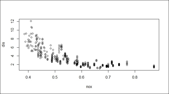
Scatter plot of variable nox against dis
2. Add the regression to the scatter plot:
3. > x = seq(0, 1, length = 500)
4. > y = predict(fit, data.frame(nox = x))
5. > lines(x, y, col = "red", lwd = 2)
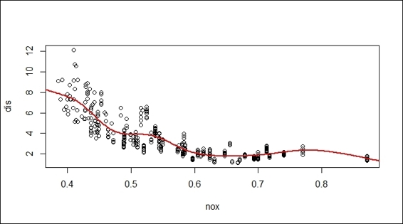
Fitted regression of gam on a scatter plot
3. Alternatively, you can plot the fitted model using the plot function:
4. > plot(fit)
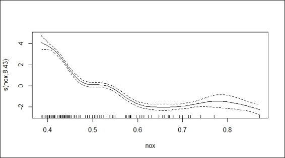
Plot of fitted gam
How it works...
To visualize the fitted regression, we first generate a scatter plot using the dis and nox variables. Then, we generate the sequence of x-axis, and respond y through the use of the predict function on the fitted model, fit. Finally, we use the lines function to add the regression line to the scatter plot.
Besides using the lines to add fitted regression lines on the scatter plot, gam has a plot function to visualize the fitted regression lines containing the confidence region. To shade the confidence region, we assign shade = TRUE within the function.
There's more...
The vis.gam function is used to produce perspective or contour plot views of the gam model predictions. It is helpful to observe how response variables interact with two predictor variables. The following is an example of a contour plot on the Boston dataset:
> fit2=gam(medv~crim+zn+crim:zn, data=Boston)
> vis.gam(fit2)
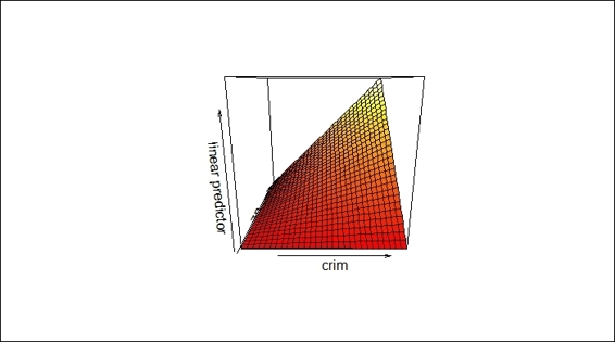
A sample contour plot produced by vis.gam
Diagnosing a generalized additive model
GAM also provides diagnostic information about the fitting procedure and results of the generalized additive model. In this recipe, we demonstrate how to plot diagnostic plots through the gam.check function.
Getting ready
Ensure that the previous recipe is completed with the gam fitted model assigned to the fit variable.
How to do it...
Perform the following step to diagnose the generalized additive model:
1. Generate the diagnostic plot using gam.check on the fitted model:
2. > gam.check(fit)
3.
4. Method: GCV Optimizer: magic
5. Smoothing parameter selection converged after 7 iterations.
6. The RMS GCV score gradient at convergence was 8.79622e-06 .
7. The Hessian was positive definite.
8. The estimated model rank was 10 (maximum possible: 10)
9. Model rank = 10 / 10
10.
11.Basis dimension (k) checking results. Low p-value (k-index<1) may
12.indicate that k is too low, especially if edf is close to k'.
13.
14. k' edf k-index p-value
15.s(nox) 9.000 8.434 0.397 0
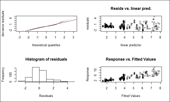
Diagnostic plot of fitted gam
How it works...
The gam.check function first produces the smoothing parameter estimation convergence information. In this example, the smoothing parameter, GCV/UBRE (Generalized Cross Validation/ Unbiased Risk Estimator) score converges after seven iterations. The mean absolute gradient of the GCV/UBRE function at the minimum is 8.79622e-06 and the estimated rank is 10. The dimension check is to test whether the basis dimension for a smooth function is adequate. From this example, the low p-value indicates that the k is set too low. One may adjust the dimension choice for smooth by specifying the argument, k, by fitting gam to the data.
In addition to providing information regarding smoothing parameter estimation convergence, the function returns four diagnostic plots. The upper-left section of the plot in the screenshot shows a quantile-comparison plot. This plot is useful to identify outliers and heavy tails. The upper-right section of the plot shows residuals versus linear predictors, which are useful in finding nonconstant error variances. The bottom-left section of the plot shows a histogram of the residuals, which is helpful in detecting non-normality. The bottom-right section shows response versus the fitted value.
There's more...
You can access the help function for more information on gam.check. In particular, this includes a detailed illustration of smoothing parameter estimation convergence and four returned plots:
> ?gam.check
In addition, more information for choose.k can be accessed by the following command:
> ?choose.k
All materials on the site are licensed Creative Commons Attribution-Sharealike 3.0 Unported CC BY-SA 3.0 & GNU Free Documentation License (GFDL)
If you are the copyright holder of any material contained on our site and intend to remove it, please contact our site administrator for approval.
© 2016-2026 All site design rights belong to S.Y.A.