Machine Learning with R Cookbook (2015)

Chapter 5. Classification (I) – Tree, Lazy, and Probabilistic

In this chapter, we will cover the following recipes:

· Preparing the training and testing datasets

· Building a classification model with recursive partitioning trees

· Visualizing a recursive partitioning tree

· Measuring the prediction performance of a recursive partitioning tree

· Pruning a recursive partitioning tree

· Building a classification model with a conditional inference tree

· Visualizing a conditional inference tree

· Measuring the prediction performance of a conditional inference tree

· Classifying data with a k-nearest neighbor classifier

· Classifying data with logistic regression

· Classifying data with the Naïve Bayes classifier

Introduction

Classification is used to identify a category of new observations (testing datasets) based on a classification model built from the training dataset, of which the categories are already known. Similar to regression, classification is categorized as a supervised learning method as it employs known answers (label) of a training dataset to predict the answer (label) of the testing dataset. The main difference between regression and classification is that regression is used to predict continuous values.

In contrast to this, classification is used to identify the category of a given observation. For example, one may use regression to predict the future price of a given stock based on historical prices. However, one should use the classification method to predict whether the stock price will rise or fall.

In this chapter, we will illustrate how to use R to perform classification. We first build a training dataset and a testing dataset from the churn dataset, and then apply different classification methods to classify the churn dataset. In the following recipes, we will introduce the tree-based classification method using a traditional classification tree and a conditional inference tree, lazy-based algorithm, and a probabilistic-based method using the training dataset to build up a classification model, and then use the model to predict the category (class label) of the testing dataset. We will also use a confusion matrix to measure the performance.

Preparing the training and testing datasets

Building a classification model requires a training dataset to train the classification model, and testing data is needed to then validate the prediction performance. In the following recipe, we will demonstrate how to split the telecom churn dataset into training and testing datasets, respectively.

Getting ready

In this recipe, we will use the telecom churn dataset as the input data source, and split the data into training and testing datasets.

How to do it...

Perform the following steps to split the churn dataset into training and testing datasets:

1. You can retrieve the churn dataset from the C50 package:

2. > install.packages("C50")

3. > library(C50)

4. > data(churn)

2. Use str to read the structure of the dataset:

3. > str(churnTrain)

3. We can remove the state, area_code, and account_length attributes, which are not appropriate for classification features:

4. > churnTrain = churnTrain[,! names(churnTrain) %in% c("state", "area_code", "account_length") ]

4. Then, split 70 percent of the data into the training dataset and 30 percent of the data into the testing dataset:

5. > set.seed(2)

6. > ind = sample(2, nrow(churnTrain), replace = TRUE, prob=c(0.7, 0.3))

7. > trainset = churnTrain[ind == 1,]

8. > testset = churnTrain[ind == 2,]

5. Lastly, use dim to explore the dimensions of both the training and testing datasets:

6. > dim(trainset)

7. [1] 2315 17

8. > dim(testset)

9. [1] 1018 17

How it works...

In this recipe, we use the telecom churn dataset as our example data source. The dataset contains 20 variables with 3,333 observations. We would like to build a classification model to predict whether a customer will churn, which is very important to the telecom company as the cost of acquiring a new customer is significantly more than retaining one.

Before building the classification model, we need to preprocess the data first. Thus, we load the churn data from the C50 package into the R session with the variable name as churn. As we determined that attributes such as state, area_code, and account_length are not useful features for building the classification model, we remove these attributes.

After preprocessing the data, we split it into training and testing datasets, respectively. We then use a sample function to randomly generate a sequence containing 70 percent of the training dataset and 30 percent of the testing dataset with a size equal to the number of observations. Then, we use a generated sequence to split the churn dataset into the training dataset, trainset, and the testing dataset, testset. Lastly, by using the dim function, we found that 2,315 out of the 3,333 observations are categorized into the training dataset, trainset, while the other 1,018 are categorized into the testing dataset, testset.

There's more...

You can combine the split process of the training and testing datasets into the split.data function. Therefore, you can easily split the data into the two datasets by calling this function and specifying the proportion and seed in the parameters:

> split.data = function(data, p = 0.7, s = 666){

+ set.seed(s)

+ index = sample(1:dim(data)[1])

+ train = data[index[1:floor(dim(data)[1] * p)], ]

+ test = data[index[((ceiling(dim(data)[1] * p)) + 1):dim(data)[1]], ]

+ return(list(train = train, test = test))

+ }

Building a classification model with recursive partitioning trees

A classification tree uses a split condition to predict class labels based on one or multiple input variables. The classification process starts from the root node of the tree; at each node, the process will check whether the input value should recursively continue to the right or left sub-branch according to the split condition, and stops when meeting any leaf (terminal) nodes of the decision tree. In this recipe, we will introduce how to apply a recursive partitioning tree on the customer churn dataset.

Getting ready

You need to have completed the previous recipe by splitting the churn dataset into the training dataset (trainset) and testing dataset (testset), and each dataset should contain exactly 17 variables.

How to do it...

Perform the following steps to split the churn dataset into training and testing datasets:

1. Load the rpart package:

2. > library(rpart)

2. Use the rpart function to build a classification tree model:

3. > churn.rp = rpart(churn ~ ., data=trainset)

3. Type churn.rp to retrieve the node detail of the classification tree:

4. > churn.rp

4. Next, use the printcp function to examine the complexity parameter:

5. > printcp(churn.rp)

6.

7. Classification tree:

8. rpart(formula = churn ~ ., data = trainset)

9.

10.Variables actually used in tree construction:

11.[1] international_plan number_customer_service_calls

12.[3] total_day_minutes total_eve_minutes

13.[5] total_intl_calls total_intl_minutes

14.[7] voice_mail_plan

15.

16.Root node error: 342/2315 = 0.14773

17.

18.n= 2315

19.

20. CP nsplit rel error xerror xstd

21.1 0.076023 0 1.00000 1.00000 0.049920

22.2 0.074561 2 0.84795 0.99708 0.049860

23.3 0.055556 4 0.69883 0.76023 0.044421

24.4 0.026316 7 0.49415 0.52632 0.037673

25.5 0.023392 8 0.46784 0.52047 0.037481

26.6 0.020468 10 0.42105 0.50877 0.037092

27.7 0.017544 11 0.40058 0.47076 0.035788

28.8 0.010000 12 0.38304 0.47661 0.035993

5. Next, use the plotcp function to plot the cost complexity parameters:

6. > plotcp(churn.rp)

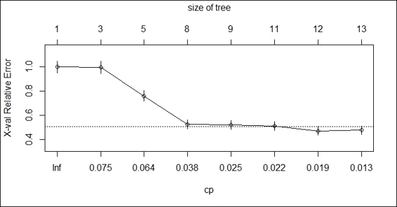
Figure 1: The cost complexity parameter plot

6. Lastly, use the summary function to examine the built model:

7. > summary(churn.rp)

How it works...

In this recipe, we use a recursive partitioning tree from the rpart package to build a tree-based classification model. The recursive portioning tree includes two processes: recursion and partitioning. During the process of decision induction, we have to consider a statistic evaluation question (or simply a yes/no question) to partition the data into different partitions in accordance with the assessment result. Then, as we have determined the child node, we can repeatedly perform the splitting until the stop criteria is satisfied.

For example, the data (shown in the following figure) in the root node can be partitioned into two groups with regard to the question of whether f1 is smaller than X. If so, the data is divided into the left-hand side. Otherwise, it is split into the right-hand side. Then, we can continue to partition the left-hand side data with the question of whether f2 is smaller than Y:

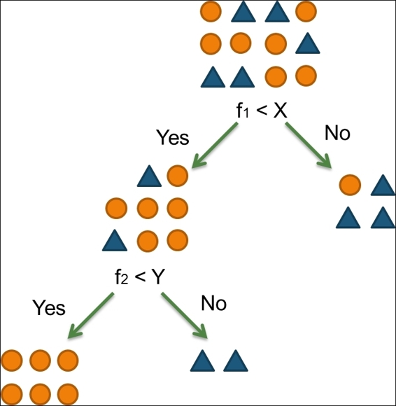
Figure 2: Recursive partioning tree

In the first step, we load the rpart package with the library function. Next, we build a classification model using the churn variable as a classification category (class label) and the remaining variables as input features.

After the model is built, you can type the variable name of the built model, churn.rp, to display the tree node details. In the printed node detail, n indicates the sample size, loss indicates the misclassification cost, yval stands for the classified membership (no or yes, in this case), and yprob stands for the probabilities of two classes (the left value refers to the probability reaching label no, and the right value refers to the probability reaching label, yes).

Then, we use the printcp function to print the complexity parameters of the built tree model. From the output of printcp, one should find the value of CP, a complexity parameter, which serves as a penalty to control the size of the tree. In short, the greater the CP value, the fewer the number of splits there are (nsplit). The output value (the rel error) represents the average deviance of the current tree divided by the average deviance of the null tree. A xerrorvalue represents the relative error estimated by a 10-fold classification. xstd stands for the standard error of the relative error.

To make the CP (cost complexity parameter) table more readable, we use plotcp to generate an information graphic of the CP table. As per the screenshot (step 5), the x-axis at the bottom illustrates the cp value, the y-axis illustrates the relative error, and the upper x-axis displays the size of the tree. The dotted line indicates the upper limit of a standard deviation. From the screenshot, we can determine that minimum cross-validation error occurs when the tree is at a size of 12.

We can also use the summary function to display the function call, complexity parameter table for the fitted tree model, variable importance, which helps identify the most important variable for the tree classification (summing up to 100), and detailed information of each node.

The advantage of using the decision tree is that it is very flexible and easy to interpret. It works on both classification and regression problems, and more; it is nonparametric. Therefore, one does not have to worry about whether the data is linear separable. As for the disadvantage of using the decision tree, it is that it tends to be biased and over-fitted. However, you can conquer the bias problem through the use of a conditional inference tree, and solve the problem of over-fitting through a random forest method or tree pruning.

See also

· For more information about the rpart, printcp, and summary functions, please use the help function:

· > ?rpart

· > ?printcp

· > ?summary.rpart

· C50 is another package that provides a decision tree and a rule-based model. If you are interested in the package, you may refer to the document at http://cran.r-project.org/web/packages/C50/C50.pdf.

Visualizing a recursive partitioning tree

From the last recipe, we learned how to print the classification tree in a text format. To make the tree more readable, we can use the plot function to obtain the graphical display of a built classification tree.

Getting ready

One needs to have the previous recipe completed by generating a classification model, and assign the model into the churn.rp variable.

How to do it...

Perform the following steps to visualize the classification tree:

1. Use the plot function and the text function to plot the classification tree:

2. > plot(churn.rp, margin= 0.1)

3. > text(churn.rp, all=TRUE, use.n = TRUE)

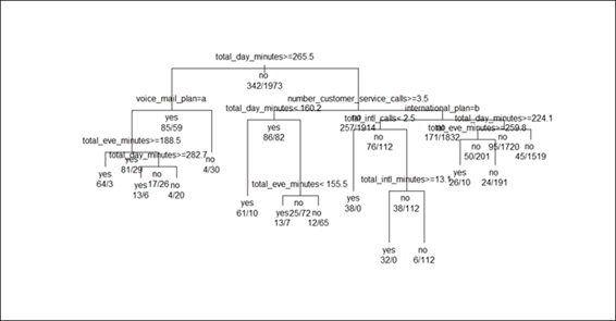
Figure 3: The graphical display of a classification tree

2. You can also specify the uniform, branch, and margin parameter to adjust the layout:

3. > plot(churn.rp, uniform=TRUE, branch=0.6, margin=0.1)

4. > text(churn.rp, all=TRUE, use.n = TRUE)

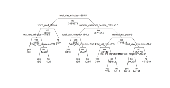
Figure 4: Adjust the layout of the classification tree

How it works...

Here, we demonstrate how to use the plot function to graphically display a classification tree. The plot function can simply visualize the classification tree, and you can then use the text function to add text to the plot.

In Figure 3, we assign margin = 0.1 as a parameter to add extra white space around the border to prevent the displayed text being truncated by the margin. It shows that the length of the branches displays the relative magnitude of the drop in deviance. We then use the text function to add labels for the nodes and branches. By default, the text function will add a split condition on each split, and add a category label in each terminal node. In order to add extra information on the tree plot, we set the parameter as all equal to TRUE to add a label to all the nodes. In addition to this, we add a parameter by specifying use.n = TRUE to add extra information, which shows that the actual number of observations fall into two different categories (no and yes).

In Figure 4, we set the option branch to 0.6 to add a shoulder to each plotted branch. In addition to this, in order to display branches of an equal length rather than relative magnitude of the drop in deviance, we set the option uniform to TRUE. As a result, Figure 4 shows a classification tree with short shoulders and branches of equal length.

See also

· You may use ?plot.rpart to read more about the plotting of the classification tree. This document also includes information on how to specify the parameters, uniform, branch, compress, nspace, margin, and minbranch, to adjust the layout of the classification tree.

Measuring the prediction performance of a recursive partitioning tree

Since we have built a classification tree in the previous recipes, we can use it to predict the category (class label) of new observations. Before making a prediction, we first validate the prediction power of the classification tree, which can be done by generating a classification table on the testing dataset. In this recipe, we will introduce how to generate a predicted label versus a real label table with the predict function and the table function, and explain how to generate a confusion matrix to measure the performance.

Getting ready

You need to have the previous recipe completed by generating the classification model, churn.rp. In addition to this, you have to prepare the training dataset, trainset, and the testing dataset, testset, generated in the first recipe of this chapter.

How to do it...

Perform the following steps to validate the prediction performance of a classification tree:

1. You can use the predict function to generate a predicted label of testing the dataset:

2. > predictions = predict(churn.rp, testset, type="class")

2. Use the table function to generate a classification table for the testing dataset:

3. > table(testset$churn, predictions)

4. predictions

5. yes no

6. yes 100 41

7. no 18 859

3. One can further generate a confusion matrix using the confusionMatrix function provided in the caret package:

4. > library(caret)

5. > confusionMatrix(table(predictions, testset$churn))

6. Confusion Matrix and Statistics

7.

8.

9. predictions yes no

10. yes 100 18

11. no 41 859

12.

13. Accuracy : 0.942

14. 95% CI : (0.9259, 0.9556)

15. No Information Rate : 0.8615

16. P-Value [Acc > NIR] : < 2.2e-16

17.

18. Kappa : 0.7393

19. Mcnemar's Test P-Value : 0.004181

20.

21. Sensitivity : 0.70922

22. Specificity : 0.97948

23. Pos Pred Value : 0.84746

24. Neg Pred Value : 0.95444

25. Prevalence : 0.13851

26. Detection Rate : 0.09823

27. Detection Prevalence : 0.11591

28. Balanced Accuracy : 0.84435

29.

30. 'Positive' Class : yes

How it works...

In this recipe, we use a predict function and built up classification model, churn.rp, to predict the possible class labels of the testing dataset, testset. The predicted categories (class labels) are coded as either no or yes. Then, we use the table function to generate a classification table on the testing dataset. From the table, we discover that there are 859 correctly predicted as no, while 18 are misclassified as yes. 100 of the yes predictions are correctly predicted, but 41 observations are misclassified into no. Further, we use the confusionMatrix function from the caret package to produce a measurement of the classification model.

See also

· You may use ?confusionMatrix to read more about the performance measurement using the confusion matrix

· For those who are interested in the definition output by the confusion matrix, please refer to the Wikipedia entry, Confusion_matrix (http://en.wikipedia.org/wiki/Confusion_matrix)

Pruning a recursive partitioning tree

In previous recipes, we have built a complex decision tree for the churn dataset. However, sometimes we have to remove sections that are not powerful in classifying instances to avoid over-fitting, and to improve the prediction accuracy. Therefore, in this recipe, we introduce the cost complexity pruning method to prune the classification tree.

Getting ready

You need to have the previous recipe completed by generating a classification model, and assign the model into the churn.rp variable.

How to do it...

Perform the following steps to prune the classification tree:

1. Find the minimum cross-validation error of the classification tree model:

2. > min(churn.rp$cptable[,"xerror"])

3. [1] 0.4707602

2. Locate the record with the minimum cross-validation errors:

3. > which.min(churn.rp$cptable[,"xerror"])

4. 7

3. Get the cost complexity parameter of the record with the minimum cross-validation errors:

4. > churn.cp = churn.rp$cptable[7,"CP"]

5. > churn.cp

6. [1] 0.01754386

4. Prune the tree by setting the cp parameter to the CP value of the record with minimum cross-validation errors:

5. > prune.tree = prune(churn.rp, cp= churn.cp)

5. Visualize the classification tree by using the plot and text function:

6. > plot(prune.tree, margin= 0.1)

7. > text(prune.tree, all=TRUE , use.n=TRUE)

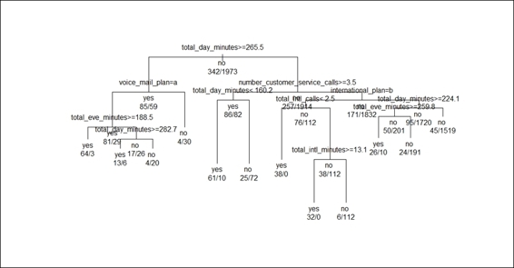
Figure 5: The pruned classification tree

6. Next, you can generate a classification table based on the pruned classification tree model:

7. > predictions = predict(prune.tree, testset, type="class")

8. > table(testset$churn, predictions)

9. predictions

10. yes no

11. yes 95 46

12. no 14 863

7. Lastly, you can generate a confusion matrix based on the classification table:

8. > confusionMatrix(table(predictions, testset$churn))

9. Confusion Matrix and Statistics

10.

11.

12.

13.predictions yes no

14. yes 95 14

15. no 46 863

16.

17. Accuracy : 0.9411

18. 95% CI : (0.9248, 0.9547)

19. No Information Rate : 0.8615

20. P-Value [Acc > NIR] : 2.786e-16

21.

22. Kappa : 0.727

23. Mcnemar's Test P-Value : 6.279e-05

24.

25. Sensitivity : 0.67376

26. Specificity : 0.98404

27. Pos Pred Value : 0.87156

28. Neg Pred Value : 0.94939

29. Prevalence : 0.13851

30. Detection Rate : 0.09332

31. Detection Prevalence : 0.10707

32. Balanced Accuracy : 0.82890

33.

34. 'Positive' Class : yes

How it works...

In this recipe, we discussed pruning a classification tree to avoid over-fitting and producing a more robust classification model. We first located the record with the minimum cross-validation errors within the cptable, and we then extracted the CP of the record and assigned the value to churn.cp. Next, we used the prune function to prune the classification tree with churn.cp as the parameter. Then, by using the plot function, we graphically displayed the pruned classification tree. From Figure 5, it is clear that the split of the tree is less than the original classification tree (Figure 3). Lastly, we produced a classification table and used the confusion matrix to validate the performance of the pruned tree. The result shows that the accuracy (0.9411) is slightly lower than the original model (0.942), and also suggests that the pruned tree may not perform better than the original classification tree as we have pruned some split conditions (Still, one should examine the change in sensitivity and specificity). However, the pruned tree model is more robust as it removes some split conditions that may lead to over-fitting.

See also

· For those who would like to know more about cost complexity pruning, please refer to the Wikipedia article for Pruning (decision_trees): http://en.wikipedia.org/wiki/Pruning_(decision_trees

Building a classification model with a conditional inference tree

In addition to traditional decision trees (rpart), conditional inference trees (ctree) are another popular tree-based classification method. Similar to traditional decision trees, conditional inference trees also recursively partition the data by performing a univariate split on the dependent variable. However, what makes conditional inference trees different from traditional decision trees is that conditional inference trees adapt the significance test procedures to select variables rather than selecting variables by maximizing information measures (rpart employs a Gini coefficient). In this recipe, we will introduce how to adapt a conditional inference tree to build a classification model.

Getting ready

You need to have the first recipe completed by generating the training dataset, trainset, and the testing dataset, testset.

How to do it...

Perform the following steps to build the conditional inference tree:

1. First, we use ctree from the party package to build the classification model:

2. > library(party)

3. > ctree.model = ctree(churn ~ . , data = trainset)

2. Then, we examine the built tree model:

3. > ctree.model

How it works...

In this recipe, we used a conditional inference tree to build a classification tree. The use of ctree is similar to rpart. Therefore, you can easily test the classification power using either a traditional decision tree or a conditional inference tree while confronting classification problems. Next, we obtain the node details of the classification tree by examining the built model. Within the model, we discover that ctree provides information similar to a splitcondition, criterion (1 – p-value), statistics (test statistics), and weight (the case weight corresponding to the node). However, it does not offer as much information as rpart does through the use of the summary function.

See also

· You may use the help function to refer to the definition of Binary Tree Class and read more about the properties of binary trees:

· > help("BinaryTree-class")

Visualizing a conditional inference tree

Similar to rpart, the party package also provides a visualization method for users to plot conditional inference trees. In the following recipe, we will introduce how to use the plot function to visualize conditional inference trees.

Getting ready

You need to have the first recipe completed by generating the conditional inference tree model, ctree.model. In addition to this, you need to have both, trainset and testset, loaded in an R session.

How to do it...

Perform the following steps to visualize the conditional inference tree:

1. Use the plot function to plot ctree.model built in the last recipe:

2. > plot(ctree.model)

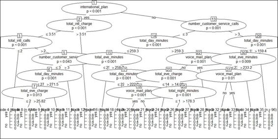
Figure 6: A conditional inference tree of churn data

2. To obtain a simple conditional inference tree, one can reduce the built model with less input features, and redraw the classification tree:

3. > daycharge.model = ctree(churn ~ total_day_charge, data = trainset)

4. > plot(daycharge.model)

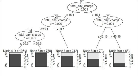
Figure 7: A conditional inference tree using the total_day_charge variable as only split condition

How it works...

To visualize the node detail of the conditional inference tree, we can apply the plot function on a built classification model. The output figure reveals that every intermediate node shows the dependent variable name and the p-value. The split condition is displayed on the left and right branches. The terminal nodes show the number of categorized observations, n, and the probability of a class label of either 0 or 1.

Taking Figure 7 as an example, we first build a classification model using total_day_charge as the only feature and churn as the class label. The built classification tree shows that when total_day_charge is above 48.18, the lighter gray area is greater than the darker gray in node 9, which indicates that the customer with a day charge of over 48.18 has a greater likelihood to churn (label = yes).

See also

· The visualization of the conditional inference tree comes from the plot.BinaryTree function. If you are interested in adjusting the layout of the classification tree, you may use the help function to read the following document:

· > ?plot.BinaryTree

Measuring the prediction performance of a conditional inference tree

After building a conditional inference tree as a classification model, we can use the treeresponse and predict functions to predict categories of the testing dataset, testset, and further validate the prediction power with a classification table and a confusion matrix.

Getting ready

You need to have the previous recipe completed by generating the conditional inference tree model, ctree.model. In addition to this, you need to have both trainset and testset loaded in an R session.

How to do it...

Perform the following steps to measure the prediction performance of a conditional inference tree:

1. You can use the predict function to predict the category of the testing dataset, testset:

2. > ctree.predict = predict(ctree.model ,testset)

3. > table(ctree.predict, testset$churn)

4.

5. ctree.predict yes no

6. yes 99 15

7. no 42 862

2. Furthermore, you can use confusionMatrix from the caret package to generate the performance measurements of the prediction result:

3. > confusionMatrix(table(ctree.predict, testset$churn))

4. Confusion Matrix and Statistics

5.

6.

7. ctree.predict yes no

8. yes 99 15

9. no 42 862

10.

11. Accuracy : 0.944

12. 95% CI : (0.9281, 0.9573)

13. No Information Rate : 0.8615

14. P-Value [Acc > NIR] : < 2.2e-16

15.

16. Kappa : 0.7449

17. Mcnemar's Test P-Value : 0.0005736

18.

19. Sensitivity : 0.70213

20. Specificity : 0.98290

21. Pos Pred Value : 0.86842

22. Neg Pred Value : 0.95354

23. Prevalence : 0.13851

24. Detection Rate : 0.09725

25. Detection Prevalence : 0.11198

26. Balanced Accuracy : 0.84251

27.

28. 'Positive' Class : yes

3. You can also use the treeresponse function, which will tell you the list of class probabilities:

4. > tr = treeresponse(ctree.model, newdata = testset[1:5,])

5. > tr

6. [[1]]

7. [1] 0.03497409 0.96502591

8.

9. [[2]]

10.[1] 0.02586207 0.97413793

11.

12.[[3]]

13.[1] 0.02586207 0.97413793

14.

15.[[4]]

16.[1] 0.02586207 0.97413793

17.

18.[[5]]

19.[1] 0.03497409 0.96502591

How it works...

In this recipe, we first demonstrate that one can use the prediction function to predict the category (class label) of the testing dataset, testset, and then employ a table function to generate a classification table. Next, you can use the confusionMatrix function built into the caret package to determine the performance measurements.

In addition to the predict function, treeresponse is also capable of estimating the class probability, which will often classify labels with a higher probability. In this example, we demonstrated how to obtain the estimated class probability using the top five records of the testing dataset, testset. The treeresponse function returns a list of five probabilities. You can use the list to determine the label of instance.

See also

· For the predict function, you can specify the type as response, prob, or node. If you specify the type as prob when using the predict function (for example, predict(… type="prob")), you will get exactly the same result as what treeresponse returns.

Classifying data with the k-nearest neighbor classifier

K-nearest neighbor (knn) is a nonparametric lazy learning method. From a nonparametric view, it does not make any assumptions about data distribution. In terms of lazy learning, it does not require an explicit learning phase for generalization. The following recipe will introduce how to apply the k-nearest neighbor algorithm on the churn dataset.

Getting ready

You need to have the previous recipe completed by generating the training and testing datasets.

How to do it...

Perform the following steps to classify the churn data with the k-nearest neighbor algorithm:

1. First, one has to install the class package and have it loaded in an R session:

2. > install.packages("class")

3. > library(class)

2. Replace yes and no of the voice_mail_plan and international_plan attributes in both the training dataset and testing dataset to 1 and 0:

3. > levels(trainset$international_plan) = list("0"="no", "1"="yes")

4. > levels(trainset$voice_mail_plan) = list("0"="no", "1"="yes")

5. > levels(testset$international_plan) = list("0"="no", "1"="yes")

6. > levels(testset$voice_mail_plan) = list("0"="no", "1"="yes")

3. Use the knn classification method on the training dataset and the testing dataset:

4. > churn.knn = knn(trainset[,! names(trainset) %in% c("churn")], testset[,! names(testset) %in% c("churn")], trainset$churn, k=3)

4. Then, you can use the summary function to retrieve the number of predicted labels:

5. > summary(churn.knn)

6. yes no

7. 77 941

5. Next, you can generate the classification matrix using the table function:

6. > table(testset$churn, churn.knn)

7. churn.knn

8. yes no

9. yes 44 97

10. no 33 844

6. Lastly, you can generate a confusion matrix by using the confusionMatrix function:

7. > confusionMatrix(table(testset$churn, churn.knn))

8. Confusion Matrix and Statistics

9.

10. churn.knn

11. yes no

12. yes 44 97

13. no 33 844

14.

15. Accuracy : 0.8723

16. 95% CI : (0.8502, 0.8922)

17. No Information Rate : 0.9244

18. P-Value [Acc > NIR] : 1

19.

20. Kappa : 0.339

21. Mcnemar's Test P-Value : 3.286e-08

22.

23. Sensitivity : 0.57143

24. Specificity : 0.89692

25. Pos Pred Value : 0.31206

26. Neg Pred Value : 0.96237

27. Prevalence : 0.07564

28. Detection Rate : 0.04322

29. Detection Prevalence : 0.13851

30. Balanced Accuracy : 0.73417

31.

32. 'Positive' Class : yes

How it works...

knn trains all samples and classifies new instances based on a similarity (distance) measure. For example, the similarity measure can be formulated as follows:

· Euclidian Distance:

· Manhattan Distance:

In knn, a new instance is classified to a label (class) that is common among the k-nearest neighbors. If k = 1, then the new instance is assigned to the class where its nearest neighbor belongs. The only required input for the algorithm is k. If we give a small k input, it may lead to over-fitting. On the other hand, if we give a large k input, it may result in under-fitting. To choose a proper k-value, one can count on cross-validation.

The advantages of knn are:

· The cost of the learning process is zero

· It is nonparametric, which means that you do not have to make the assumption of data distribution

· You can classify any data whenever you can find similarity measures of given instances

The main disadvantages of knn are:

· It is hard to interpret the classified result.

· It is an expensive computation for a large dataset.

· The performance relies on the number of dimensions. Therefore, for a high dimension problem, you should reduce the dimension first to increase the process performance.

The use of knn does not vary significantly from applying a tree-based algorithm mentioned in the previous recipes. However, while a tree-based algorithm may show you the decision tree model, the output produced by knn only reveals classification category factors. However, before building a classification model, one should replace the attribute with a string type to an integer since the k-nearest neighbor algorithm needs to calculate the distance between observations. Then, we build up a classification model by specifying k=3, which means choosing the three nearest neighbors. After the classification model is built, we can generate a classification table using predicted factors and the testing dataset label as the input. Lastly, we can generate a confusion matrix from the classification table. The confusion matrix output reveals an accuracy result of (0.8723), which suggests that both the tree-based methods mentioned in previous recipes outperform the accuracy of the k-nearest neighbor classification method in this case. Still, we cannot determine which model is better depending merely on accuracy, one should also examine the specificity and sensitivity from the output.

See also

· There is another package named kknn, which provides a weighted k-nearest neighbor classification, regression, and clustering. You can learn more about the package by reading this document: http://cran.r-project.org/web/packages/kknn/kknn.pdf.

Classifying data with logistic regression

Logistic regression is a form of probabilistic statistical classification model, which can be used to predict class labels based on one or more features. The classification is done by using the logit function to estimate the outcome probability. One can use logistic regression by specifying the family as a binomial while using the glm function. In this recipe, we will introduce how to classify data using logistic regression.

Getting ready

You need to have completed the first recipe by generating training and testing datasets.

How to do it...

Perform the following steps to classify the churn data with logistic regression:

1. With the specification of family as a binomial, we apply the glm function on the dataset, trainset, by using churn as a class label and the rest of the variables as input features:

2. > fit = glm(churn ~ ., data = trainset, family=binomial)

2. Use the summary function to obtain summary information of the built logistic regression model:

3. > summary(fit)

4.

5. Call:

6. glm(formula = churn ~ ., family = binomial, data = trainset)

7.

8. Deviance Residuals:

9. Min 1Q Median 3Q Max

10.-3.1519 0.1983 0.3460 0.5186 2.1284

11.

12.Coefficients:

13. Estimate Std. Error z value Pr(>|z|)

14.(Intercept) 8.3462866 0.8364914 9.978 < 2e-16

15.international_planyes -2.0534243 0.1726694 -11.892 < 2e-16

16.voice_mail_planyes 1.3445887 0.6618905 2.031 0.042211

17.number_vmail_messages -0.0155101 0.0209220 -0.741 0.458496

18.total_day_minutes 0.2398946 3.9168466 0.061 0.951163

19.total_day_calls -0.0014003 0.0032769 -0.427 0.669141

20.total_day_charge -1.4855284 23.0402950 -0.064 0.948592

21.total_eve_minutes 0.3600678 1.9349825 0.186 0.852379

22.total_eve_calls -0.0028484 0.0033061 -0.862 0.388928

23.total_eve_charge -4.3204432 22.7644698 -0.190 0.849475

24.total_night_minutes 0.4431210 1.0478105 0.423 0.672367

25.total_night_calls 0.0003978 0.0033188 0.120 0.904588

26.total_night_charge -9.9162795 23.2836376 -0.426 0.670188

27.total_intl_minutes 0.4587114 6.3524560 0.072 0.942435

28.total_intl_calls 0.1065264 0.0304318 3.500 0.000464

29.total_intl_charge -2.0803428 23.5262100 -0.088 0.929538

30.number_customer_service_calls -0.5109077 0.0476289 -10.727 < 2e-16

31.

32.(Intercept) ***

33.international_planyes ***

34.voice_mail_planyes *

35.number_vmail_messages

36.total_day_minutes

37.total_day_calls

38.total_day_charge

39.total_eve_minutes

40.total_eve_calls

41.total_eve_charge

42.total_night_minutes

43.total_night_calls

44.total_night_charge

45.total_intl_minutes

46.total_intl_calls ***

47.total_intl_charge

48.number_customer_service_calls ***

49.---

50.Signif. codes: 0 '***' 0.001 '**' 0.01 '*' 0.05 '.' 0.1 ' ' 1

51.

52.(Dispersion parameter for binomial family taken to be 1)

53.

54. Null deviance: 1938.8 on 2314 degrees of freedom

55.Residual deviance: 1515.3 on 2298 degrees of freedom

56.AIC: 1549.3

57.

58.Number of Fisher Scoring iterations: 6

3. Then, we find that the built model contains insignificant variables, which would lead to misclassification. Therefore, we use significant variables only to train the classification model:

4. > fit = glm(churn ~ international_plan + voice_mail_plan+total_intl_calls+number_customer_service_calls, data = trainset, family=binomial)

5. > summary(fit)

6.

7. Call:

8. glm(formula = churn ~ international_plan + voice_mail_plan +

9. total_intl_calls + number_customer_service_calls, family = binomial,

10. data = trainset)

11.

12.Deviance Residuals:

13. Min 1Q Median 3Q Max

14.-2.7308 0.3103 0.4196 0.5381 1.6716

15.

16.Coefficients:

17. Estimate Std. Error z value

18.(Intercept) 2.32304 0.16770 13.852

19.international_planyes -2.00346 0.16096 -12.447

20.voice_mail_planyes 0.79228 0.16380 4.837

21.total_intl_calls 0.08414 0.02862 2.939

22.number_customer_service_calls -0.44227 0.04451 -9.937

23. Pr(>|z|)

24.(Intercept) < 2e-16 ***

25.international_planyes < 2e-16 ***

26.voice_mail_planyes 1.32e-06 ***

27.total_intl_calls 0.00329 **

28.number_customer_service_calls < 2e-16 ***

29.---

30.Signif. codes:

31.0 es: des: **rvice_calls < '. es: de

32.

33.(Dispersion parameter for binomial family taken to be 1)

34.

35. Null deviance: 1938.8 on 2314 degrees of freedom

36.Residual deviance: 1669.4 on 2310 degrees of freedom

37.AIC: 1679.4

38.

39.Number of Fisher Scoring iterations: 5

4. Then, you can then use a fitted model, fit, to predict the outcome of testset. You can also determine the class by judging whether the probability is above 0.5:

5. > pred = predict(fit,testset, type="response")

6. > Class = pred >.5

5. Next, the use of the summary function will show you the binary outcome count, and reveal whether the probability is above 0.5:

6. > summary(Class)

7. Mode FALSE TRUE NA's

8. logical 29 989 0

6. You can generate the counting statistics based on the testing dataset label and predicted result:

7. > tb = table(testset$churn,Class)

8. > tb
 Class

9. FALSE TRUE

10. yes 18 123

11. no 11 866

7. You can turn the statistics of the previous step into a classification table, and then generate the confusion matrix:

8. > churn.mod = ifelse(testset$churn == "yes", 1, 0)

9. > pred_class = churn.mod

10.> pred_class[pred<=.5] = 1- pred_class[pred<=.5]

11.> ctb = table(churn.mod, pred_class)

12.> ctb

13. pred_class

14.churn.mod 0 1

15. 0 866 11

16. 1 18 123

17.> confusionMatrix(ctb)

18.Confusion Matrix and Statistics

19.

20. pred_class

21.churn.mod 0 1

22. 0 866 11

23. 1 18 123

24.

25. Accuracy : 0.9715

26. 95% CI : (0.9593, 0.9808)

27. No Information Rate : 0.8684

28. P-Value [Acc > NIR] : <2e-16

29.

30. Kappa : 0.8781

31. Mcnemar's Test P-Value : 0.2652

32.

33. Sensitivity : 0.9796

34. Specificity : 0.9179

35. Pos Pred Value : 0.9875

36. Neg Pred Value : 0.8723

37. Prevalence : 0.8684

38. Detection Rate : 0.8507

39. Detection Prevalence : 0.8615

40. Balanced Accuracy : 0.9488

41.

42. 'Positive' Class : 0

How it works...

Logistic regression is very similar to linear regression; the main difference is that the dependent variable in linear regression is continuous, but the dependent variable in logistic regression is dichotomous (or nominal). The primary goal of logistic regression is to use logit to yield the probability of a nominal variable is related to the measurement variable. We can formulate logit in following equation: ln(P/(1-P)), where P is the probability that certain event occurs.

The advantage of logistic regression is that it is easy to interpret, it directs model logistic probability, and provides a confidence interval for the result. Unlike the decision tree, which is hard to update the model, you can quickly update the classification model to incorporate new data in logistic regression. The main drawback of the algorithm is that it suffers from multicollinearity and, therefore, the explanatory variables must be linear independent. glmprovides a generalized linear regression model, which enables specifying the model in the option family. If the family is specified to a binomial logistic, you can set the family as a binomial to classify the dependent variable of the category.

The classification process begins by generating a logistic regression model with the use of the training dataset by specifying Churn as the class label, the other variables as training features, and family set as binomial. We then use the summary function to generate the model's summary information. From the summary information, we may find some insignificant variables (p-values > 0.05), which may lead to misclassification. Therefore, we should consider only significant variables for the model.

Next, we use the fit function to predict the categorical dependent variable of the testing dataset, testset. The fit function outputs the probability of a class label, with a result equal to 0.5 and below, suggesting that the predicted label does not match the label of the testing dataset, and a probability above 0.5 indicates that the predicted label matches the label of the testing dataset. Further, we can use the summary function to obtain the statistics of whether the predicted label matches the label of the testing dataset. Lastly, in order to generate a confusion matrix, we first generate a classification table, and then use confusionMatrix to generate the performance measurement.

See also

· For more information of how to use the glm function, please refer to Chapter 4, Understanding Regression Analysis, which covers how to interpret the output of the glm function

Classifying data with the Naïve Bayes classifier

The Naïve Bayes classifier is also a probability-based classifier, which is based on applying the Bayes theorem with a strong independent assumption. In this recipe, we will introduce how to classify data with the Naïve Bayes classifier.

Getting ready

You need to have the first recipe completed by generating training and testing datasets.

How to do it...

Perform the following steps to classify the churn data with the Naïve Bayes classifier:

1. Load the e1071 library and employ the naiveBayes function to build the classifier:

2. > library(e1071)

3. > classifier=naiveBayes(trainset[, !names(trainset) %in% c("churn")], trainset$churn)

2. Type classifier to examine the function call, a-priori probability, and conditional probability:

3. > classifier

4.

5. Naive Bayes Classifier for Discrete Predictors

6.

7. Call:

8. naiveBayes.default(x = trainset[, !names(trainset) %in% c("churn")],

9. y = trainset$churn)

10.

11.A-priori probabilities:

12.trainset$churn

13. yes no

14.0.1477322 0.8522678

15.

16.Conditional probabilities:

17. international_plan

18.trainset$churn no yes

19. yes 0.70467836 0.29532164

20. no 0.93512418 0.06487582

3. Next, you can generate a classification table for the testing dataset:

4. > bayes.table = table(predict(classifier, testset[, !names(testset) %in% c("churn")]), testset$churn)

5. > bayes.table

6.

7. yes no

8. yes 68 45

9. no 73 832

4. Lastly, you can generate a confusion matrix from the classification table:

5. > confusionMatrix(bayes.table)

6. Confusion Matrix and Statistics

7.

8.

9. yes no

10. yes 68 45

11. no 73 832

12.

13. Accuracy : 0.8841

14. 95% CI : (0.8628, 0.9031)

15. No Information Rate : 0.8615

16. P-Value [Acc > NIR] : 0.01880

17.

18. Kappa : 0.4701

19. Mcnemar's Test P-Value : 0.01294

20.

21. Sensitivity : 0.4823

22. Specificity : 0.9487

23. Pos Pred Value : 0.6018

24. Neg Pred Value : 0.9193

25. Prevalence : 0.1385

26. Detection Rate : 0.0668

27. Detection Prevalence : 0.1110

28. Balanced Accuracy : 0.7155

29.

30. 'Positive' Class : yes

How it works...

Naive Bayes assumes that features are conditionally independent, which the effect of a predictor(x) to class (c) is independent of the effect of other predictors to class(c). It computes the posterior probability, P(c|x), as the following formula:

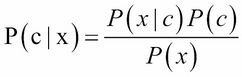
Where P(x|c) is called likelihood, p(x) is called the marginal likelihood, and p(c) is called the prior probability. If there are many predictors, we can formulate the posterior probability as follows:

The advantage of Naïve Bayes is that it is relatively simple and straightforward to use. It is suitable when the training set is relative small, and may contain some noisy and missing data. Moreover, you can easily obtain the probability for a prediction. The drawbacks of Naïve Bayes are that it assumes that all features are independent and equally important, which is very unlikely in real-world cases.

In this recipe, we use the Naïve Bayes classifier from the e1071 package to build a classification model. First, we specify all the variables (excluding the churn class label) as the first input parameters, and specify the churn class label as the second parameter in the naiveBayes function call. Next, we assign the classification model into the variable classifier. Then, we print the variable classifier to obtain information, such as function call, A-priori probabilities, and conditional probabilities. We can also use the predict function to obtain the predicted outcome and the table function to retrieve the classification table of the testing dataset. Finally, we use a confusion matrix to calculate the performance measurement of the classification model.

At last, we list a comparison table of all the mentioned algorithms in this chapter:

See also

· To learn more about the Bayes theorem, you can refer to the following Wikipedia article: http://en.wikipedia.org/wiki/Bayes'_theorem