Machine Learning with R Cookbook (2015)
Chapter 6. Classification (II) – Neural Network and SVM
In this chapter, we will cover the following recipes:
· Classifying data with a support vector machine
· Choosing the cost of a support vector machine
· Visualizing an SVM fit
· Predicting labels based on a model trained by a support vector machine
· Tuning a support vector machine
· Training a neural network with neuralnet
· Visualizing a neural network trained by neuralnet
· Predicting labels based on a model trained by neuralnet
· Training a neural network with nnet
· Predicting labels based on a model trained by nnet
Introduction
Most research has shown that support vector machines (SVM) and neural networks (NN) are powerful classification tools, which can be applied to several different areas. Unlike tree-based or probabilistic-based methods that were mentioned in the previous chapter, the process of how support vector machines and neural networks transform from input to output is less clear and can be hard to interpret. As a result, both support vector machines and neural networks are referred to as black box methods.
The development of a neural network is inspired by human brain activities. As such, this type of network is a computational model that mimics the pattern of the human mind. In contrast to this, support vector machines first map input data into a high dimension feature space defined by the kernel function, and find the optimum hyperplane that separates the training data by the maximum margin. In short, we can think of support vector machines as a linear algorithm in a high dimensional space.
Both these methods have advantages and disadvantages in solving classification problems. For example, support vector machine solutions are the global optimum, while neural networks may suffer from multiple local optimums. Thus, choosing between either depends on the characteristics of the dataset source. In this chapter, we will illustrate the following:
· How to train a support vector machine
· Observing how the choice of cost can affect the SVM classifier
· Visualizing the SVM fit
· Predicting the labels of a testing dataset based on the model trained by SVM
· Tuning the SVM
In the neural network section, we will cover:
· How to train a neural network
· How to visualize a neural network model
· Predicting the labels of a testing dataset based on a model trained by neuralnet
· Finally, we will show how to train a neural network with nnet, and how to use it to predict the labels of a testing dataset
Classifying data with a support vector machine
The two most well known and popular support vector machine tools are libsvm and SVMLite. For R users, you can find the implementation of libsvm in the e1071 package and SVMLite in the klaR package. Therefore, you can use the implemented function of these two packages to train support vector machines. In this recipe, we will focus on using the svm function (the libsvm implemented version) from the e1071 package to train a support vector machine based on the telecom customer churn data training dataset.
Getting ready
In this recipe, we will continue to use the telecom churn dataset as the input data source to train the support vector machine. For those who have not prepared the dataset, please refer to Chapter 5, Classification (I) – Tree, Lazy, and Probabilistic, for details.
How to do it...
Perform the following steps to train the SVM:
1. Load the e1071 package:
2. > library(e1071)
2. Train the support vector machine using the svm function with trainset as the input dataset, and use churn as the classification category:
3. > model = svm(churn~., data = trainset, kernel="radial", cost=1, gamma = 1/ncol(trainset))
3. Finally, you can obtain overall information about the built model with summary:
4. > summary(model)
5.
6. Call:
7. svm(formula = churn ~ ., data = trainset, kernel = "radial", cost = 1, gamma = 1/ncol(trainset))
8.
9.
10.Parameters:
11. SVM-Type: C-classification
12. SVM-Kernel: radial
13. cost: 1
14. gamma: 0.05882353
15.
16.Number of Support Vectors: 691
17.
18. ( 394 297 )
19.
20.
21.Number of Classes: 2
22.
23.Levels:
24. yes no
How it works...
The support vector machine constructs a hyperplane (or set of hyperplanes) that maximize the margin width between two classes in a high dimensional space. In these, the cases that define the hyperplane are support vectors, as shown in the following figure:
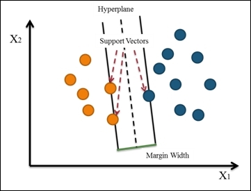
Figure 1: Support Vector Machine
Support vector machine starts from constructing a hyperplane that maximizes the margin width. Then, it extends the definition to a nonlinear separable problem. Lastly, it maps the data to a high dimensional space where the data can be more easily separated with a linear boundary.
The advantage of using SVM is that it builds a highly accurate model through an engineering problem-oriented kernel. Also, it makes use of the regularization term to avoid over-fitting. It also does not suffer from local optimal and multicollinearity. The main limitation of SVM is its speed and size in the training and testing time. Therefore, it is not suitable or efficient enough to construct classification models for data that is large in size. Also, since it is hard to interpret SVM, how does the determination of the kernel take place? Regularization is another problem that we need tackle.
In this recipe, we continue to use the telecom churn dataset as our example data source. We begin training a support vector machine using libsvm provided in the e1071 package. Within the training function, svm, one can specify the kernel function, cost, and the gamma function. For the kernel argument, the default value is radial, and one can specify the kernel to a linear, polynomial, radial basis, and sigmoid. As for the gamma argument, the default value is equal to (1/data dimension), and it controls the shape of the separating hyperplane. Increasing the gamma argument usually increases the number of support vectors.
As for the cost, the default value is set to 1, which indicates that the regularization term is constant, and the larger the value, the smaller the margin is. We will discuss more on how the cost can affect the SVM classifier in the next recipe. Once the support vector machine is built, the summary function can be used to obtain information, such as calls, parameters, number of classes, and the types of label.
See also
Another popular support vector machine tool is SVMLight. Unlike the e1071 package, which provides the full implementation of libsvm, the klaR package simply provides an interface to SVMLight only. To use SVMLight, one can perform the following steps:
1. Install the klaR package:
2. > install.packages("klaR")
3. > library(klaR)
2. Download the SVMLight source code and binary for your platform from http://svmlight.joachims.org/. For example, if your guest OS is Windows 64-bit, you should download the file from http://download.joachims.org/svm_light/current/svm_light_windows64.zip.
3. Then, you should unzip the file and put the workable binary in the working directory; you may check your working directory by using the getwd function:
4. > getwd()
4. Train the support vector machine using the svmlight function:
5. > model.light = svmlight(churn~., data = trainset, kernel="radial", cost=1, gamma = 1/ncol(trainset))
Choosing the cost of a support vector machine
The support vector machines create an optimum hyperplane that separates the training data by the maximum margin. However, sometimes we would like to allow some misclassifications while separating categories. The SVM model has a cost function, which controls training errors and margins. For example, a small cost creates a large margin (a soft margin) and allows more misclassifications. On the other hand, a large cost creates a narrow margin (a hard margin) and permits fewer misclassifications. In this recipe, we will illustrate how the large and small cost will affect the SVM classifier.
Getting ready
In this recipe, we will use the iris dataset as our example data source.
How to do it...
Perform the following steps to generate two different classification examples with different costs:
1. Subset the iris dataset with columns named as Sepal.Length, Sepal.Width, Species, with species in setosa and virginica:
2. > iris.subset = subset(iris, select=c("Sepal.Length", "Sepal.Width", "Species"), Species %in% c("setosa","virginica"))
2. Then, you can generate a scatter plot with Sepal.Length as the x-axis and the Sepal.Width as the y-axis:
3. > plot(x=iris.subset$Sepal.Length,y=iris.subset$Sepal.Width, col=iris.subset$Species, pch=19)
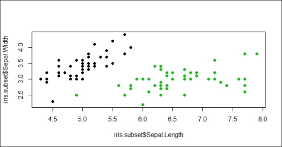
Figure 2: Scatter plot of Sepal.Length and Sepal.Width with subset of iris dataset
3. Next, you can train SVM based on iris.subset with the cost equal to 1:
4. > svm.model = svm(Species ~ ., data=iris.subset, kernel='linear', cost=1, scale=FALSE)
4. Then, we can circle the support vector with blue circles:
5. > points(iris.subset[svm.model$index,c(1,2)],col="blue",cex=2)
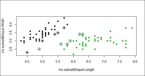
Figure 3: Circling support vectors with blue ring
5. Lastly, we can add a separation line on the plot:
6. > w = t(svm.model$coefs) %*% svm.model$SV
7. > b = -svm.model$rho
8. > abline(a=-b/w[1,2], b=-w[1,1]/w[1,2], col="red", lty=5)
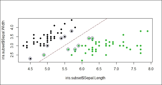
Figure 4: Add separation line to scatter plot
6. In addition to this, we create another SVM classifier where cost = 10,000:
7. > plot(x=iris.subset$Sepal.Length,y=iris.subset$Sepal.Width, col=iris.subset$Species, pch=19)
8. > svm.model = svm(Species ~ ., data=iris.subset, type='C-classification', kernel='linear', cost=10000, scale=FALSE)
9. > points(iris.subset[svm.model$index,c(1,2)],col="blue",cex=2)
10.> w = t(svm.model$coefs) %*% svm.model$SV
11.> b = -svm.model$rho
12.> abline(a=-b/w[1,2], b=-w[1,1]/w[1,2], col="red", lty=5)
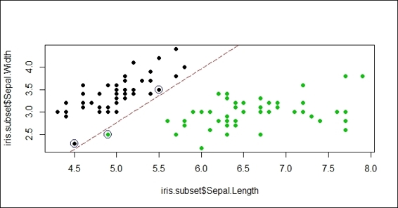
Figure 5: A classification example with large cost
How it works...
In this recipe, we demonstrate how different costs can affect the SVM classifier. First, we create an iris subset with the columns, Sepal.Length, Sepal.Width, and Species containing the species, setosa and virginica. Then, in order to create a soft margin and allow some misclassification, we use an SVM with small cost (where cost = 1) to train the support of the vector machine. Next, we circle the support vectors with blue circles and add the separation line. As per Figure 5, one of the green points (virginica) is misclassified (it is classified to setosa) to the other side of the separation line due to the choice of the small cost.
In addition to this, we would like to determine how a large cost can affect the SVM classifier. Therefore, we choose a large cost (where cost = 10,000). From Figure 5, we can see that the margin created is narrow (a hard margin) and no misclassification cases are present. As a result, the two examples show that the choice of different costs may affect the margin created and also affect the possibilities of misclassification.
See also
· The idea of soft margin, which allows misclassified examples, was suggested by Corinna Cortes and Vladimir N. Vapnik in 1995 in the following paper: Cortes, C., and Vapnik, V. (1995). Support-vector networks. Machine learning, 20(3), 273-297.
Visualizing an SVM fit
To visualize the built model, one can first use the plot function to generate a scatter plot of data input and the SVM fit. In this plot, support vectors and classes are highlighted through the color symbol. In addition to this, one can draw a contour filled plot of the class regions to easily identify misclassified samples from the plot.
Getting ready
In this recipe, we will use two datasets: the iris dataset and the telecom churn dataset. For the telecom churn dataset, one needs to have completed the previous recipe by training a support vector machine with SVM, and to have saved the SVM fit model.
How to do it...
Perform the following steps to visualize the SVM fit object:
1. Use SVM to train the support vector machine based on the iris dataset, and use the plot function to visualize the fitted model:
2. > data(iris)
3. > model.iris = svm(Species~., iris)
4. > plot(model.iris, iris, Petal.Width ~ Petal.Length, slice = list(Sepal.Width = 3, Sepal.Length = 4))
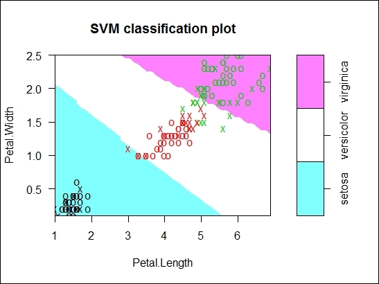
Figure 6: The SVM classification plot of trained SVM fit based on iris dataset
2. Visualize the SVM fit object, model, using the plot function with the dimensions of total_day_minutes and total_intl_charge:
3. > plot(model, trainset, total_day_minutes ~ total_intl_charge)
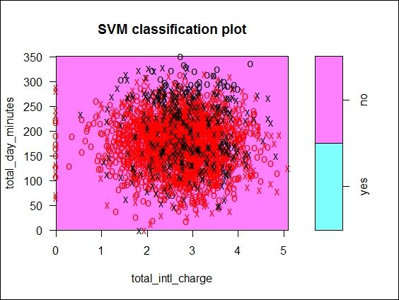
Figure 7: The SVM classification plot of trained SVM fit based on churn dataset
How it works...
In this recipe, we demonstrate how to use the plot function to visualize the SVM fit. In the first plot, we train a support vector machine using the iris dataset. Then, we use the plot function to visualize the fitted SVM.
In the argument list, we specify the fitted model in the first argument and the dataset (this should be the same data used to build the model) as the second parameter. The third parameter indicates the dimension used to generate the classification plot. By default, the plot function can only generate a scatter plot based on two dimensions (for the x-axis and y-axis). Therefore, we select the variables, Petal.Length and Petal.Width as the two dimensions to generate the scatter plot.
From Figure 6, we find Petal.Length assigned to the x-axis, Petal.Width assigned to the y-axis, and data points with X and O symbols scattered on the plot. Within the scatter plot, the X symbol shows the support vector and the Osymbol represents the data points. These two symbols can be altered through the configuration of the svSymbol and dataSymbol options. Both the support vectors and true classes are highlighted and colored depending on their label (green refers to viginica, red refers to versicolor, and black refers to setosa). The last argument, slice, is set when there are more than two variables. Therefore, in this example, we use the additional variables, Sepal.width and Sepal.length, by assigning a constant of 3 and 4.
Next, we take the same approach to draw the SVM fit based on customer churn data. In this example, we use total_day_minutes and total_intl_charge as the two dimensions used to plot the scatterplot. As per Figure 7, the support vectors and data points in red and black are scattered closely together in the central region of the plot, and there is no simple way to separate them.
See also
· There are other parameters, such as fill, grid, symbolPalette, and so on, that can be configured to change the layout of the plot. You can use the help function to view the following document for further information:
· > ?svm.plot
Predicting labels based on a model trained by a support vector machine
In the previous recipe, we trained an SVM based on the training dataset. The training process finds the optimum hyperplane that separates the training data by the maximum margin. We can then utilize the SVM fit to predict the label (category) of new observations. In this recipe, we will demonstrate how to use the predict function to predict values based on a model trained by SVM.
Getting ready
You need to have completed the previous recipe by generating a fitted SVM, and save the fitted model in model.
How to do it...
Perform the following steps to predict the labels of the testing dataset:
1. Predict the label of the testing dataset based on the fitted SVM and attributes of the testing dataset:
2. > svm.pred = predict(model, testset[, !names(testset) %in% c("churn")])
2. Then, you can use the table function to generate a classification table with the prediction result and labels of the testing dataset:
3. > svm.table=table(svm.pred, testset$churn)
4. > svm.table
5.
6. svm.pred yes no
7. yes 70 12
8. no 71 865
3. Next, you can use classAgreement to calculate coefficients compared to the classification agreement:
4. > classAgreement(svm.table)
5. $diag
6. [1] 0.9184676
7.
8. $kappa
9. [1] 0.5855903
10.
11.$rand
12.[1] 0.850083
13.
14.$crand
15.[1] 0.5260472
4. Now, you can use confusionMatrix to measure the prediction performance based on the classification table:
5. > library(caret)
6. > confusionMatrix(svm.table)
7. Confusion Matrix and Statistics
8.
9.
10.svm.pred yes no
11. yes 70 12
12. no 71 865
13.
14. Accuracy : 0.9185
15. 95% CI : (0.8999, 0.9345)
16. No Information Rate : 0.8615
17. P-Value [Acc > NIR] : 1.251e-08
18.
19. Kappa : 0.5856
20. Mcnemar's Test P-Value : 1.936e-10
21.
22. Sensitivity : 0.49645
23. Specificity : 0.98632
24. Pos Pred Value : 0.85366
25. Neg Pred Value : 0.92415
26. Prevalence : 0.13851
27. Detection Rate : 0.06876
28. Detection Prevalence : 0.08055
29. Balanced Accuracy : 0.74139
30.
31. 'Positive' Class : yes
How it works...
In this recipe, we first used the predict function to obtain the predicted labels of the testing dataset. Next, we used the table function to generate the classification table based on the predicted labels of the testing dataset. So far, the evaluation procedure is very similar to the evaluation process mentioned in the previous chapter.
We then introduced a new function, classAgreement, which computes several coefficients of agreement between the columns and rows of a two-way contingency table. The coefficients include diag, kappa, rand, and crand. The diagcoefficient represents the percentage of data points in the main diagonal of the classification table, kappa refers to diag, which is corrected for an agreement by a change (the probability of random agreements), rand represents the Rand index, which measures the similarity between two data clusters, and crand indicates the Rand index, which is adjusted for the chance grouping of elements.
Finally, we used confusionMatrix from the caret package to measure the performance of the classification model. The accuracy of 0.9185 shows that the trained support vector machine can correctly classify most of the observations. However, accuracy alone is not a good measurement of a classification model. One should also reference sensitivity and specificity.
There's more...
Besides using SVM to predict the category of new observations, you can use SVM to predict continuous values. In other words, one can use SVM to perform regression analysis.
In the following example, we will show how to perform a simple regression prediction based on a fitted SVM with the type specified as eps-regression.
Perform the following steps to train a regression model with SVM:
1. Train a support vector machine based on a Quartet dataset:
2. > library(car)
3. > data(Quartet)
4. > model.regression = svm(Quartet$y1~Quartet$x,type="eps-regression")
2. Use the predict function to obtain prediction results:
3. > predict.y = predict(model.regression, Quartet$x)
4. > predict.y
5. 1 2 3 4 5 6 7 8
6. 8.196894 7.152946 8.807471 7.713099 8.533578 8.774046 6.186349 5.763689
7. 9 10 11
8. 8.726925 6.621373 5.882946
3. Plot the predicted points as squares and the training data points as circles on the same plot:
4. > plot(Quartet$x, Quartet$y1, pch=19)
5. > points(Quartet$x, predict.y, pch=15, col="red")
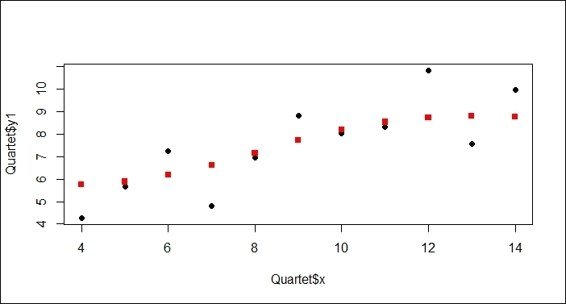
Figure 8: The scatter plot contains predicted data points and training data points
Tuning a support vector machine
Besides using different feature sets and the kernel function in support vector machines, one trick that you can use to tune its performance is to adjust the gamma and cost configured in the argument. One possible approach to test the performance of different gamma and cost combination values is to write a for loop to generate all the combinations of gamma and cost as inputs to train different support vector machines. Fortunately, SVM provides a tuning function, tune.svm, which makes the tuning much easier. In this recipe, we will demonstrate how to tune a support vector machine through the use of tune.svm.
Getting ready
You need to have completed the previous recipe by preparing a training dataset, trainset.
How to do it...
Perform the following steps to tune the support vector machine:
1. First, tune the support vector machine using tune.svm:
2. > tuned = tune.svm(churn~., data = trainset, gamma = 10^(-6:-1), cost = 10^(1:2))
2. Next, you can use the summary function to obtain the tuning result:
3. > summary(tuned)
4.
5. Parameter tuning of 'svm':
6.
7. - sampling method: 10-fold cross validation
8.
9. - best parameters:
10. gamma cost
11. 0.01 100
12.
13.- best performance: 0.08077885
14.
15.- Detailed performance results:
16. gamma cost error dispersion
17.1 1e-06 10 0.14774780 0.02399512
18.2 1e-05 10 0.14774780 0.02399512
19.3 1e-04 10 0.14774780 0.02399512
20.4 1e-03 10 0.14774780 0.02399512
21.5 1e-02 10 0.09245223 0.02046032
22.6 1e-01 10 0.09202306 0.01938475
23.7 1e-06 100 0.14774780 0.02399512
24.8 1e-05 100 0.14774780 0.02399512
25.9 1e-04 100 0.14774780 0.02399512
26.10 1e-03 100 0.11794484 0.02368343
27.11 1e-02 100 0.08077885 0.01858195
28.12 1e-01 100 0.12356135 0.01661508
3. After retrieving the best performance parameter from tuning the result, you can retrain the support vector machine with the best performance parameter:
4. > model.tuned = svm(churn~., data = trainset, gamma = tuned$best.parameters$gamma, cost = tuned$best.parameters$cost)
5. > summary(model.tuned)
6.
7. Call:
8. svm(formula = churn ~ ., data = trainset, gamma = 10^-2, cost = 100)
9.
10.
11.Parameters:
12. SVM-Type: C-classification
13. SVM-Kernel: radial
14. cost: 100
15. gamma: 0.01
16.
17.Number of Support Vectors: 547
18.
19. ( 304 243 )
20.
21.
22.Number of Classes: 2
23.
24.Levels:
25. yes no
4. Then, you can use the predict function to predict labels based on the fitted SVM:
5. > svm.tuned.pred = predict(model.tuned, testset[, !names(testset) %in% c("churn")])
5. Next, generate a classification table based on the predicted and original labels of the testing dataset:
6. > svm.tuned.table=table(svm.tuned.pred, testset$churn)
7. > svm.tuned.table
8.
9. svm.tuned.pred yes no
10. yes 95 24
11. no 46 853
6. Also, generate a class agreement to measure the performance:
7. > classAgreement(svm.tuned.table)
8. $diag
9. [1] 0.9312377
10.
11.$kappa
12.[1] 0.691678
13.
14.$rand
15.[1] 0.871806
16.
17.$crand
18.[1] 0.6303615
7. Finally, you can use a confusion matrix to measure the performance of the retrained model:
8. > confusionMatrix(svm.tuned.table)
9. Confusion Matrix and Statistics
10.
11.
12.svm.tuned.pred yes no
13. yes 95 24
14. no 46 853
15.
16. Accuracy : 0.9312
17. 95% CI : (0.9139, 0.946)
18. No Information Rate : 0.8615
19. P-Value [Acc > NIR] : 1.56e-12
20.
21. Kappa : 0.6917
22. Mcnemar's Test P-Value : 0.01207
23.
24. Sensitivity : 0.67376
25. Specificity : 0.97263
26. Pos Pred Value : 0.79832
27. Neg Pred Value : 0.94883
28. Prevalence : 0.13851
29. Detection Rate : 0.09332
30. Detection Prevalence : 0.11690
31. Balanced Accuracy : 0.82320
32.
33. 'Positive' Class : yes
How it works...
To tune the support vector machine, you can use a trial and error method to find the best gamma and cost parameters. In other words, one has to generate a variety of combinations of gamma and cost for the purpose of training different support vector machines.
In this example, we generate different gamma values from 10^-6 to 10^-1, and cost with a value of either 10 or 100. Therefore, you can use the tuning function, svm.tune, to generate 12 sets of parameters. The function then makes 10 cross-validations and outputs the error dispersion of each combination. As a result, the combination with the least error dispersion is regarded as the best parameter set. From the summary table, we found that gamma with a value of 0.01 and cost with a value of 100 are the best parameters for the SVM fit.
After obtaining the best parameters, we can then train a new support vector machine with gamma equal to 0.01 and cost equal to 100. Additionally, we can obtain a classification table based on the predicted labels and labels of the testing dataset. We can also obtain a confusion matrix from the classification table. From the output of the confusion matrix, you can determine the accuracy of the newly trained model in comparison to the original model.
See also
· For more information about how to tune SVM with svm.tune, you can use the help function to access this document:
· > ?svm.tune
Training a neural network with neuralnet
The neural network is constructed with an interconnected group of nodes, which involves the input, connected weights, processing element, and output. Neural networks can be applied to many areas, such as classification, clustering, and prediction. To train a neural network in R, you can use neuralnet, which is built to train multilayer perceptron in the context of regression analysis, and contains many flexible functions to train forward neural networks. In this recipe, we will introduce how to use neuralnet to train a neural network.
Getting ready
In this recipe, we will use an iris dataset as our example dataset. We will first split the iris dataset into a training and testing datasets, respectively.
How to do it...
Perform the following steps to train a neural network with neuralnet:
1. First load the iris dataset and split the data into training and testing datasets:
2. > data(iris)
3. > ind = sample(2, nrow(iris), replace = TRUE, prob=c(0.7, 0.3))
4. > trainset = iris[ind == 1,]
5. > testset = iris[ind == 2,]
2. Then, install and load the neuralnet package:
3. > install.packages("neuralnet")
4. > library(neuralnet)
3. Add the columns versicolor, setosa, and virginica based on the name matched value in the Species column:
4. > trainset$setosa = trainset$Species == "setosa"
5. > trainset$virginica = trainset$Species == "virginica"
6. > trainset$versicolor = trainset$Species == "versicolor"
4. Next, train the neural network with the neuralnet function with three hidden neurons in each layer. Notice that the results may vary with each training, so you might not get the same result. However, you can use set.seed at the beginning, so you can get the same result in every training process
5. > network = neuralnet(versicolor + virginica + setosa~ Sepal.Length + Sepal.Width + Petal.Length + Petal.Width, trainset, hidden=3)
6. > network
7. Call: neuralnet(formula = versicolor + virginica + setosa ~ Sepal.Length + Sepal.Width + Petal.Length + Petal.Width, data = trainset, hidden = 3)
8.
9. 1 repetition was calculated.
10.
11. Error Reached Threshold Steps
12.1 0.8156100175 0.009994274769 11063
5. Now, you can view the summary information by accessing the result.matrix attribute of the built neural network model:
6. > network$result.matrix
7. 1
8. error 0.815610017474
9. reached.threshold 0.009994274769
10.steps 11063.000000000000
11.Intercept.to.1layhid1 1.686593311644
12.Sepal.Length.to.1layhid1 0.947415215237
13.Sepal.Width.to.1layhid1 -7.220058260187
14.Petal.Length.to.1layhid1 1.790333443486
15.Petal.Width.to.1layhid1 9.943109233330
16.Intercept.to.1layhid2 1.411026063895
17.Sepal.Length.to.1layhid2 0.240309549505
18.Sepal.Width.to.1layhid2 0.480654059973
19.Petal.Length.to.1layhid2 2.221435192437
20.Petal.Width.to.1layhid2 0.154879347818
21.Intercept.to.1layhid3 24.399329878242
22.Sepal.Length.to.1layhid3 3.313958088512
23.Sepal.Width.to.1layhid3 5.845670010464
24.Petal.Length.to.1layhid3 -6.337082722485
25.Petal.Width.to.1layhid3 -17.990352566695
26.Intercept.to.versicolor -1.959842102421
27.1layhid.1.to.versicolor 1.010292389835
28.1layhid.2.to.versicolor 0.936519720978
29.1layhid.3.to.versicolor 1.023305801833
30.Intercept.to.virginica -0.908909982893
31.1layhid.1.to.virginica -0.009904635231
32.1layhid.2.to.virginica 1.931747950462
33.1layhid.3.to.virginica -1.021438938226
34.Intercept.to.setosa 1.500533827729
35.1layhid.1.to.setosa -1.001683936613
36.1layhid.2.to.setosa -0.498758815934
37.1layhid.3.to.setosa -0.001881935696
6. Lastly, you can view the generalized weight by accessing it in the network:
7. > head(network$generalized.weights[[1]])
How it works...
The neural network is a network made up of artificial neurons (or nodes). There are three types of neurons within the network: input neurons, hidden neurons, and output neurons. In the network, neurons are connected; the connection strength between neurons is called weights. If the weight is greater than zero, it is in an excitation status. Otherwise, it is in an inhibition status. Input neurons receive the input information; the higher the input value, the greater the activation. Then, the activation value is passed through the network in regard to weights and transfer functions in the graph. The hidden neurons (or output neurons) then sum up the activation values and modify the summed values with the transfer function. The activation value then flows through hidden neurons and stops when it reaches the output nodes. As a result, one can use the output value from the output neurons to classify the data.
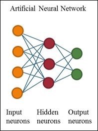
Figure 9: Artificial Neural Network
The advantages of a neural network are: first, it can detect nonlinear relationships between the dependent and independent variable. Second, one can efficiently train large datasets using the parallel architecture. Third, it is a nonparametric model so that one can eliminate errors in the estimation of parameters. The main disadvantages of a neural network are that it often converges to the local minimum rather than the global minimum. Also, it might over-fit when the training process goes on for too long.
In this recipe, we demonstrate how to train a neural network. First, we split the iris dataset into training and testing datasets, and then install the neuralnet package and load the library into an R session. Next, we add the columns versicolor, setosa, and virginica based on the name matched value in the Species column, respectively. We then use the neuralnet function to train the network model. Besides specifying the label (the column where the name equals to versicolor, virginica, and setosa) and training attributes in the function, we also configure the number of hidden neurons (vertices) as three in each layer.
Then, we examine the basic information about the training process and the trained network saved in the network. From the output message, it shows the training process needed 11,063 steps until all the absolute partial derivatives of the error function were lower than 0.01 (specified in the threshold). The error refers to the likelihood of calculating Akaike Information Criterion (AIC). To see detailed information on this, you can access the result.matrix of the built neural network to see the estimated weight. The output reveals that the estimated weight ranges from -18 to 24.40; the intercepts of the first hidden layer are 1.69, 1.41 and 24.40, and the two weights leading to the first hidden neuron are estimated as 0.95 (Sepal.Length), -7.22 (Sepal.Width), 1.79 (Petal.Length), and 9.94 (Petal.Width). We can lastly determine that the trained neural network information includes generalized weights, which express the effect of each covariate. In this recipe, the model generates 12 generalized weights, which are the combination of four covariates (Sepal.Length, Sepal.Width, Petal.Length, Petal.Width) to three responses (setosa, virginica, versicolor).
See also
· For a more detailed introduction on neuralnet, one can refer to the following paper: Günther, F., and Fritsch, S. (2010). neuralnet: Training of neural networks. The R journal, 2(1), 30-38.
Visualizing a neural network trained by neuralnet
The package, neuralnet, provides the plot function to visualize a built neural network and the gwplot function to visualize generalized weights. In following recipe, we will cover how to use these two functions.
Getting ready
You need to have completed the previous recipe by training a neural network and have all basic information saved in the network.
How to do it...
Perform the following steps to visualize the neural network and the generalized weights:
1. You can visualize the trained neural network with the plot function:
2. > plot(network)
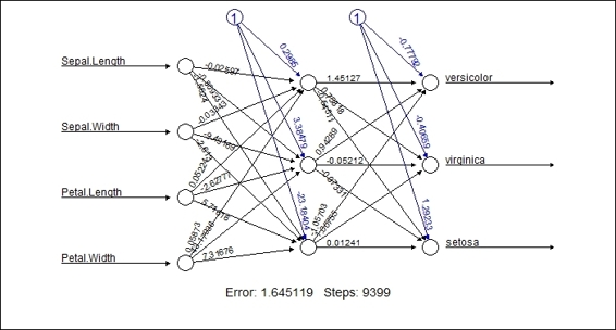
Figure 10: The plot of the trained neural network
2. Furthermore, you can use gwplot to visualize the generalized weights:
3. > par(mfrow=c(2,2))
4. > gwplot(network,selected.covariate="Petal.Width")
5. > gwplot(network,selected.covariate="Sepal.Width")
6. > gwplot(network,selected.covariate="Petal.Length")
7. > gwplot(network,selected.covariate="Petal.Width")
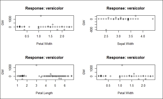
Figure 11: The plot of generalized weights
How it works...
In this recipe, we demonstrate how to visualize the trained neural network and the generalized weights of each trained attribute. As per Figure 10, the plot displays the network topology of the trained neural network. Also, the plot includes the estimated weight, intercepts and basic information about the training process. At the bottom of the figure, one can find the overall error and number of steps required to converge.
Figure 11 presents the generalized weight plot in regard to network$generalized.weights. The four plots in Figure 11 display the four covariates: Petal.Width, Sepal.Width, Petal.Length, and Petal.Width, in regard to the versicolor response. If all the generalized weights are close to zero on the plot, it means the covariate has little effect. However, if the overall variance is greater than one, it means the covariate has a nonlinear effect.
See also
· For more information about gwplot, one can use the help function to access the following document:
· > ?gwplot
Predicting labels based on a model trained by neuralnet
Similar to other classification methods, we can predict the labels of new observations based on trained neural networks. Furthermore, we can validate the performance of these networks through the use of a confusion matrix. In the following recipe, we will introduce how to use the compute function in a neural network to obtain a probability matrix of the testing dataset labels, and use a table and confusion matrix to measure the prediction performance.
Getting ready
You need to have completed the previous recipe by generating the training dataset, trainset, and the testing dataset, testset. The trained neural network needs to be saved in the network.
How to do it...
Perform the following steps to measure the prediction performance of the trained neural network:
1. First, generate a prediction probability matrix based on a trained neural network and the testing dataset, testset:
2. > net.predict = compute(network, testset[-5])$net.result
2. Then, obtain other possible labels by finding the column with the greatest probability:
3. > net.prediction = c("versicolor", "virginica", "setosa")[apply(net.predict, 1, which.max)]
3. Generate a classification table based on the predicted labels and the labels of the testing dataset:
4. > predict.table = table(testset$Species, net.prediction)
5. > predict.table
6. prediction
7. setosa versicolor virginica
8. setosa 20 0 0
9. versicolor 0 19 1
10. virginica 0 2 16
4. Next, generate classAgreement from the classification table:
5. > classAgreement(predict.table)
6. $diag
7. [1] 0.9444444444
8.
9. $kappa
10.[1] 0.9154488518
11.
12.$rand
13.[1] 0.9224318658
14.
15.$crand
16.[1] 0.8248251737
5. Finally, use confusionMatrix to measure the prediction performance:
6. > confusionMatrix(predict.table)
7. Confusion Matrix and Statistics
8.
9. prediction
10. setosa versicolor virginica
11. setosa 20 0 0
12. versicolor 0 19 1
13. virginica 0 2 16
14.
15.Overall Statistics
16.
17. Accuracy : 0.9482759
18. 95% CI : (0.8561954, 0.9892035)
19. No Information Rate : 0.362069
20. P-Value [Acc > NIR] : < 0.00000000000000022204
21.
22. Kappa : 0.922252
23. Mcnemar's Test P-Value : NA
24.
25.Statistics by Class:
26.
27. Class: setosa Class: versicolor Class: virginica
28.Sensitivity 1.0000000 0.9047619 0.9411765
29.Specificity 1.0000000 0.9729730 0.9512195
30.Pos Pred Value 1.0000000 0.9500000 0.8888889
31.Neg Pred Value 1.0000000 0.9473684 0.9750000
32.Prevalence 0.3448276 0.3620690 0.2931034
33.Detection Rate 0.3448276 0.3275862 0.2758621
34.Detection Prevalence 0.3448276 0.3448276 0.3103448
35.Balanced Accuracy 1.0000000 0.9388674 0.9461980
How it works...
In this recipe, we demonstrate how to predict labels based on a model trained by neuralnet. Initially, we use the compute function to create an output probability matrix based on the trained neural network and the testing dataset. Then, to convert the probability matrix to class labels, we use the which.max function to determine the class label by selecting the column with the maximum probability within the row. Next, we use a table to generate a classification matrix based on the labels of the testing dataset and the predicted labels. As we have created the classification table, we can employ a confusion matrix to measure the prediction performance of the built neural network.
See also
· In this recipe, we use the net.result function, which is the overall result of the neural network, used to predict the labels of the testing dataset. Apart from examining the overall result by accessing net.result, the computefunction also generates the output from neurons in each layer. You can examine the output of neurons to get a better understanding of how compute works:
· > compute(network, testset[-5])
Training a neural network with nnet
The nnet package is another package that can deal with artificial neural networks. This package provides the functionality to train feed-forward neural networks with traditional back propagation. As you can find most of the neural network function implemented in the neuralnet package, in this recipe we provide a short overview of how to train neural networks with nnet.
Getting ready
In this recipe, we do not use the trainset and trainset generated from the previous step; please reload the iris dataset again.
How to do it...
Perform the following steps to train the neural network with nnet:
1. First, install and load the nnet package:
2. > install.packages("nnet")
3. > library(nnet)
2. Next, split the dataset into training and testing datasets:
3. > data(iris)
4. > set.seed(2)
5. > ind = sample(2, nrow(iris), replace = TRUE, prob=c(0.7, 0.3))
6. > trainset = iris[ind == 1,]
7. > testset = iris[ind == 2,]
3. Then, train the neural network with nnet:
4. > iris.nn = nnet(Species ~ ., data = trainset, size = 2, rang = 0.1, decay = 5e-4, maxit = 200)
5. # weights: 19
6. initial value 165.086674
7. iter 10 value 70.447976
8. iter 20 value 69.667465
9. iter 30 value 69.505739
10.iter 40 value 21.588943
11.iter 50 value 8.691760
12.iter 60 value 8.521214
13.iter 70 value 8.138961
14.iter 80 value 7.291365
15.iter 90 value 7.039209
16.iter 100 value 6.570987
17.iter 110 value 6.355346
18.iter 120 value 6.345511
19.iter 130 value 6.340208
20.iter 140 value 6.337271
21.iter 150 value 6.334285
22.iter 160 value 6.333792
23.iter 170 value 6.333578
24.iter 180 value 6.333498
25.final value 6.333471
26.converged
4. Use the summary to obtain information about the trained neural network:
5. > summary(iris.nn)
6. a 4-2-3 network with 19 weights
7. options were - softmax modelling decay=0.0005
8. b->h1 i1->h1 i2->h1 i3->h1 i4->h1
9. -0.38 -0.63 -1.96 3.13 1.53
10. b->h2 i1->h2 i2->h2 i3->h2 i4->h2
11. 8.95 0.52 1.42 -1.98 -3.85
12. b->o1 h1->o1 h2->o1
13. 3.08 -10.78 4.99
14. b->o2 h1->o2 h2->o2
15. -7.41 6.37 7.18
16. b->o3 h1->o3 h2->o3
17. 4.33 4.42 -12.16
How it works...
In this recipe, we demonstrate steps to train a neural network model with the nnet package. We first use nnet to train the neural network. With this function, we can set the classification formula, source of data, number of hidden units in the size parameter, initial random weight in the rang parameter, parameter for weight decay in the decay parameter, and the maximum iteration in the maxit parameter. As we set maxit to 200, the training process repeatedly runs till the value of the fitting criterion plus the decay term converge. Finally, we use the summary function to obtain information about the built neural network, which reveals that the model is built with 4-2-3 networks with 19 weights. Also, the model shows a list of weight transitions from one node to another at the bottom of the printed message.
See also
For those who are interested in the background theory of nnet and how it is made, please refer to the following articles:
· Ripley, B. D. (1996) Pattern Recognition and Neural Networks. Cambridge
· Venables, W. N., and Ripley, B. D. (2002). Modern applied statistics with S. Fourth edition. Springer
Predicting labels based on a model trained by nnet
As we have trained a neural network with nnet in the previous recipe, we can now predict the labels of the testing dataset based on the trained neural network. Furthermore, we can assess the model with a confusion matrix adapted from the caret package.
Getting ready
You need to have completed the previous recipe by generating the training dataset, trainset, and the testing dataset, testset, from the iris dataset. The trained neural network also needs to be saved as iris.nn.
How to do it...
Perform the following steps to predict labels based on the trained neural network:
1. Generate the predictions of the testing dataset based on the model, iris.nn:
2. > iris.predict = predict(iris.nn, testset, type="class")
2. Generate a classification table based on the predicted labels and labels of the testing dataset:
3. > nn.table = table(testset$Species, iris.predict)
4. iris.predict
5. setosa versicolor virginica
6. setosa 17 0 0
7. versicolor 0 14 0
8. virginica 0 1 14
3. Lastly, generate a confusion matrix based on the classification table:
4. > confusionMatrix(nn.table)
5. Confusion Matrix and Statistics
6.
7. iris.predict
8. setosa versicolor virginica
9. setosa 17 0 0
10. versicolor 0 14 0
11. virginica 0 1 14
12.
13.Overall Statistics
14.
15. Accuracy : 0.9782609
16. 95% CI : (0.8847282, 0.9994498)
17. No Information Rate : 0.3695652
18. P-Value [Acc > NIR] : < 0.00000000000000022204
19.
20. Kappa : 0.9673063
21. Mcnemar's Test P-Value : NA
22.
23.Statistics by Class:
24.
25. Class: setosa Class: versicolor
26.Sensitivity 1.0000000 0.9333333
27.Specificity 1.0000000 1.0000000
28.Pos Pred Value 1.0000000 1.0000000
29.Neg Pred Value 1.0000000 0.9687500
30.Prevalence 0.3695652 0.3260870
31.Detection Rate 0.3695652 0.3043478
32.Detection Prevalence 0.3695652 0.3043478
33.Balanced Accuracy 1.0000000 0.9666667
34. Class: virginica
35.Sensitivity 1.0000000
36.Specificity 0.9687500
37.Pos Pred Value 0.9333333
38.Neg Pred Value 1.0000000
39.Prevalence 0.3043478
40.Detection Rate 0.3043478
41.Detection Prevalence 0.3260870
42.Balanced Accuracy 0.9843750
How it works...
Similar to other classification methods, one can also predict labels based on the neural networks trained by nnet. First, we use the predict function to generate the predicted labels based on a testing dataset, testset. Within the predict function, we specify the type argument to the class, so the output will be class labels instead of a probability matrix. Next, we use the table function to generate a classification table based on predicted labels and labels written in the testing dataset. Finally, as we have created the classification table, we can employ a confusion matrix from the caret package to measure the prediction performance of the trained neural network.
See also
· For the predict function, if the type argument to class is not specified, by default, it will generate a probability matrix as a prediction result, which is very similar to net.result generated from the compute function within the neuralnet package:
· > head(predict(iris.nn, testset))
All materials on the site are licensed Creative Commons Attribution-Sharealike 3.0 Unported CC BY-SA 3.0 & GNU Free Documentation License (GFDL)
If you are the copyright holder of any material contained on our site and intend to remove it, please contact our site administrator for approval.
© 2016-2026 All site design rights belong to S.Y.A.