Machine Learning with R Cookbook (2015)
Chapter 7. Model Evaluation
In this chapter, we will cover the following topics:
· Estimating model performance with k-fold cross-validation
· Performing cross-validation with the e1071 package
· Performing cross-validation with the caret package
· Ranking the variable importance with the caret package
· Ranking the variable importance with the rminer package
· Finding highly correlated features with the caret package
· Selecting features using the caret package
· Measuring the performance of a regression model
· Measuring the prediction performance with the confusion matrix
· Measuring the prediction performance using ROCR
· Comparing an ROC curve using the caret package
· Measuring performance differences between models with the caret package
Introduction
Model evaluation is performed to ensure that a fitted model can accurately predict responses for future or unknown subjects. Without model evaluation, we might train models that over-fit in the training data. To prevent overfitting, we can employ packages, such as caret, rminer, and rocr to evaluate the performance of the fitted model. Furthermore, model evaluation can help select the optimum model, which is more robust and can accurately predict responses for future subjects.
In the following chapter, we will discuss how one can implement a simple R script or use one of the packages (for example, caret or rminer) to evaluate the performance of a fitted model.
Estimating model performance with k-fold cross-validation
The k-fold cross-validation technique is a common technique used to estimate the performance of a classifier as it overcomes the problem of over-fitting. For k-fold cross-validation, the method does not use the entire dataset to build the model, instead it splits the data into a training dataset and a testing dataset. Therefore, the model built with a training dataset can then be used to assess the performance of the model on the testing dataset. By performing n repeats of the k-fold validation, we can then use the average of n accuracies to truly assess the performance of the built model. In this recipe, we will illustrate how to perform a k-fold cross-validation.
Getting ready
In this recipe, we will continue to use the telecom churn dataset as the input data source to train the support vector machine. For those who have not prepared the dataset, please refer to Chapter 5, Classification (I) – Tree, Lazy, and Probabilistic, for detailed information.
How to do it...
Perform the following steps to cross-validate the telecom churn dataset:
1. Split the index into 10 fold using the cut function:
2. > ind = cut(1:nrow(churnTrain), breaks=10, labels=F)
2. Next, use for loop to perform a 10 fold cross-validation, repeated 10 times:
3. > accuracies = c()
4. > for (i in 1:10) {
5. + fit = svm(churn ~., churnTrain[ind != i,])
6. + predictions = predict(fit, churnTrain[ind == i, ! names(churnTrain) %in% c("churn")])
7. + correct_count = sum(predictions == churnTrain[ind == i,c("churn")])
8. + accuracies = append(correct_count / nrow(churnTrain[ind == i,]), accuracies)
9. + }
3. You can then print the accuracies:
4. > accuracies
5. [1] 0.9341317 0.8948949 0.8978979 0.9459459 0.9219219 0.9281437 0.9219219 0.9249249 0.9189189 0.9251497
4. Lastly, you can generate average accuracies with the mean function:
5. > mean(accuracies)
6. [1] 0.9213852
How it works...
In this recipe, we implement a simple script performing 10-fold cross-validations. We first generate an index with 10 fold with the cut function. Then, we implement a for loop to perform a 10-fold cross-validation 10 times. Within the loop, we first apply svm on 9 folds of data as the training set. We then use the fitted model to predict the label of the rest of the data (the testing dataset). Next, we use the sum of the correctly predicted labels to generate the accuracy. As a result of this, the loop stores 10 generated accuracies. Finally, we use the mean function to retrieve the average of the accuracies.
There's more...
If you wish to perform the k-fold validation with the use of other models, simply replace the line to generate the variable fit to whatever classifier you prefer. For example, if you would like to assess the Naïve Bayes model with a 10-fold cross-validation, you just need to replace the calling function from svm to naiveBayes:
> for (i in 1:10) {
+ fit = naiveBayes(churn ~., churnTrain[ind != i,])
+ predictions = predict(fit, churnTrain[ind == i, ! names(churnTrain) %in% c("churn")])
+ correct_count = sum(predictions == churnTrain[ind == i,c("churn")])
+ accuracies = append(correct_count / nrow(churnTrain[ind == i,]), accuracies)
+ }
Performing cross-validation with the e1071 package
Besides implementing a loop function to perform the k-fold cross-validation, you can use the tuning function (for example, tune.nnet, tune.randomForest, tune.rpart, tune.svm, and tune.knn.) within the e1071 package to obtain the minimum error value. In this recipe, we will illustrate how to use tune.svm to perform the 10-fold cross-validation and obtain the optimum classification model.
Getting ready
In this recipe, we continue to use the telecom churn dataset as the input data source to perform 10-fold cross-validation.
How to do it...
Perform the following steps to retrieve the minimum estimation error using cross-validation:
1. Apply tune.svm on the training dataset, trainset, with the 10-fold cross-validation as the tuning control. (If you find an error message, such as could not find function predict.func, please clear the workspace, restart the R session and reload the e1071 library again):
2. > tuned = tune.svm(churn~., data = trainset, gamma = 10^-2, cost = 10^2, tunecontrol=tune.control(cross=10))
2. Next, you can obtain the summary information of the model, tuned:
3. > summary(tuned)
4.
5. Error estimation of 'svm' using 10-fold cross validation: 0.08164651
3. Then, you can access the performance details of the tuned model:
4. > tuned$performances
5. gamma cost error dispersion
6. 1 0.01 100 0.08164651 0.02437228
4. Lastly, you can use the optimum model to generate a classification table:
5. > svmfit = tuned$best.model
6. > table(trainset[,c("churn")], predict(svmfit))
7.
8. yes no
9. yes 234 108
10. no 13 1960
How it works...
The e1071 package provides miscellaneous functions to build and assess models, therefore, you do not need to reinvent the wheel to evaluate a fitted model. In this recipe, we use the tune.svm function to tune the svm model with the given formula, dataset, gamma, cost, and control functions. Within the tune.control options, we configure the option as cross=10, which performs a 10-fold cross validation during the tuning process. The tuning process will eventually return the minimum estimation error, performance detail, and the best model during the tuning process. Therefore, we can obtain the performance measures of the tuning and further use the optimum model to generate a classification table.
See also
· In the e1071 package, the tune function uses a grid search to tune parameters. For those interested in other tuning functions, use the help function to view the tune document:
· > ?e1071::tune
Performing cross-validation with the caret package
The Caret (classification and regression training) package contains many functions in regard to the training process for regression and classification problems. Similar to the e1071 package, it also contains a function to perform the k-fold cross validation. In this recipe, we will demonstrate how to the perform k-fold cross validation using the caret package.
Getting ready
In this recipe, we will continue to use the telecom churn dataset as the input data source to perform the k-fold cross validation.
How to do it...
Perform the following steps to perform the k-fold cross-validation with the caret package:
1. First, set up the control parameter to train with the 10-fold cross validation in 3 repetitions:
2. > control = trainControl(method="repeatedcv", number=10, repeats=3)
2. Then, you can train the classification model on telecom churn data with rpart:
3. > model = train(churn~., data=trainset, method="rpart", preProcess="scale", trControl=control)
3. Finally, you can examine the output of the generated model:
4. > model
5. CART
6.
7. 2315 samples
8. 16 predictor
9. 2 classes: 'yes', 'no'
10.
11.Pre-processing: scaled
12.Resampling: Cross-Validated (10 fold, repeated 3 times)
13.
14.Summary of sample sizes: 2084, 2083, 2082, 2084, 2083, 2084, ...
15.
16.Resampling results across tuning parameters:
17.
18. cp Accuracy Kappa Accuracy SD Kappa SD
19. 0.0556 0.904 0.531 0.0236 0.155
20. 0.0746 0.867 0.269 0.0153 0.153
21. 0.0760 0.860 0.212 0.0107 0.141
22.
23.Accuracy was used to select the optimal model using the largest value.
24.The final value used for the model was cp = 0.05555556.
How it works...
In this recipe, we demonstrate how convenient it is to conduct the k-fold cross-validation using the caret package. In the first step, we set up the training control and select the option to perform the 10-fold cross-validation in three repetitions. The process of repeating the k-fold validation is called repeated k-fold validation, which is used to test the stability of the model. If the model is stable, one should get a similar test result. Then, we apply rpart on the training dataset with the option to scale the data and to train the model with the options configured in the previous step.
After the training process is complete, the model outputs three resampling results. Of these results, the model with cp=0.05555556 has the largest accuracy value (0.904), and is therefore selected as the optimal model for classification.
See also
· You can configure the resampling function in trainControl, in which you can specify boot, boot632, cv, repeatedcv, LOOCV, LGOCV, none, oob, adaptive_cv, adaptive_boot, or adaptive_LGOCV. To view more detailed information of how to choose the resampling method, view the trainControl document:
· > ?trainControl
Ranking the variable importance with the caret package
After building a supervised learning model, we can estimate the importance of features. This estimation employs a sensitivity analysis to measure the effect on the output of a given model when the inputs are varied. In this recipe, we will show you how to rank the variable importance with the caret package.
Getting ready
You need to have completed the previous recipe by storing the fitted rpart object in the model variable.
How to do it...
Perform the following steps to rank the variable importance with the caret package:
1. First, you can estimate the variable importance with the varImp function:
2. > importance = varImp(model, scale=FALSE)
3. > importance
4. rpart variable importance
5.
6. Overall
7. number_customer_service_calls 116.015
8. total_day_minutes 106.988
9. total_day_charge 100.648
10.international_planyes 86.789
11.voice_mail_planyes 25.974
12.total_eve_charge 23.097
13.total_eve_minutes 23.097
14.number_vmail_messages 19.885
15.total_intl_minutes 6.347
16.total_eve_calls 0.000
17.total_day_calls 0.000
18.total_night_charge 0.000
19.total_intl_calls 0.000
20.total_intl_charge 0.000
21.total_night_minutes 0.000
22.total_night_calls 0.000
2. Then, you can generate the variable importance plot with the plot function:
3. > plot(importance)
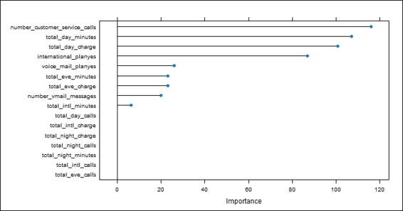
Figure 1: The visualization of variable importance using the caret package
How it works...
In this recipe, we first use the varImp function to retrieve the variable importance and obtain the summary. The overall results show the sensitivity measure of each attribute. Next, we plot the variable importance in terms of rank, which shows that the number_customer_service_calls attribute is the most important variable in the sensitivity measure.
There's more...
In some classification packages, such as rpart, the object generated from the training model contains the variable importance. We can examine the variable importance by accessing the output object:
> library(rpart)
> model.rp = rpart(churn~., data=trainset)
> model.rp$variable.importance
total_day_minutes total_day_charge
111.645286 110.881583
number_customer_service_calls total_intl_minutes
58.486651 48.283228
total_intl_charge total_eve_charge
47.698379 47.166646
total_eve_minutes international_plan
47.166646 42.194508
total_intl_calls number_vmail_messages
36.730344 19.884863
voice_mail_plan total_night_calls
19.884863 7.195828
total_eve_calls total_night_charge
3.553423 1.754547
total_night_minutes total_day_calls
1.754547 1.494986
Ranking the variable importance with the rminer package
Besides using the caret package to generate variable importance, you can use the rminer package to generate the variable importance of a classification model. In the following recipe, we will illustrate how to use rminer to obtain the variable importance of a fitted model.
Getting ready
In this recipe, we will continue to use the telecom churn dataset as the input data source to rank the variable importance.
How to do it...
Perform the following steps to rank the variable importance with rminer:
1. Install and load the package, rminer:
2. > install.packages("rminer")
3. > library(rminer)
2. Fit the svm model with the training set:
3. > model=fit(churn~.,trainset,model="svm")
3. Use the Importance function to obtain the variable importance:
4. > VariableImportance=Importance(model,trainset,method="sensv")
4. Plot the variable importance ranked by the variance:
5. > L=list(runs=1,sen=t(VariableImportance$imp),sresponses=VariableImportance$sresponses)
6. > mgraph(L,graph="IMP",leg=names(trainset),col="gray",Grid=10)
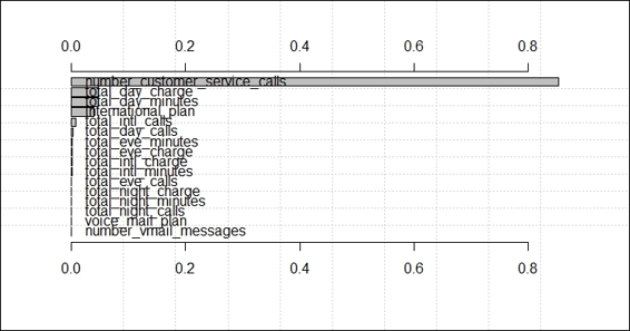
Figure 2: The visualization of variable importance using the rminer package
How it works...
Similar to the caret package, the rminer package can also generate the variable importance of a classification model. In this recipe, we first train the svm model on the training dataset, trainset, with the fit function. Then, we use the Importance function to rank the variable importance with a sensitivity measure. Finally, we use mgraph to plot the rank of the variable importance. Similar to the result obtained from using the caret package, number_customer_service_calls is the most important variable in the measure of sensitivity.
See also
· The rminer package provides many classification models for one to choose from. If you are interested in using models other than svm, you can view these options with the following command:
· > ?rminer::fit
Finding highly correlated features with the caret package
When performing regression or classification, some models perform better if highly correlated attributes are removed. The caret package provides the findCorrelation function, which can be used to find attributes that are highly correlated to each other. In this recipe, we will demonstrate how to find highly correlated features using the caret package.
Getting ready
In this recipe, we will continue to use the telecom churn dataset as the input data source to find highly correlated features.
How to do it...
Perform the following steps to find highly correlated attributes:
1. Remove the features that are not coded in numeric characters:
2. > new_train = trainset[,! names(churnTrain) %in% c("churn", "international_plan", "voice_mail_plan")]
2. Then, you can obtain the correlation of each attribute:
3. >cor_mat = cor(new_train)
3. Next, we use findCorrelation to search for highly correlated attributes with a cut off equal to 0.75:
4. > highlyCorrelated = findCorrelation(cor_mat, cutoff=0.75)
4. We then obtain the name of highly correlated attributes:
5. > names(new_train)[highlyCorrelated]
6. [1] "total_intl_minutes" "total_day_charge" "total_eve_minutes" "total_night_minutes"
How it works...
In this recipe, we search for highly correlated attributes using the caret package. In order to retrieve the correlation of each attribute, one should first remove nonnumeric attributes. Then, we perform correlation to obtain a correlation matrix. Next, we use findCorrelation to find highly correlated attributes with the cut off set to 0.75. We finally obtain the names of highly correlated (with a correlation coefficient over 0.75) attributes, which are total_intl_minutes, total_day_charge, total_eve_minutes, and total_night_minutes. You can consider removing some highly correlated attributes and keep one or two attributes for better accuracy.
See also
· In addition to the caret package, you can use the leaps, genetic, and anneal functions in the subselect package to achieve the same goal
Selecting features using the caret package
The feature selection method searches the subset of features with minimized predictive errors. We can apply feature selection to identify which attributes are required to build an accurate model. The caret package provides a recursive feature elimination function, rfe, which can help automatically select the required features. In the following recipe, we will demonstrate how to use the caret package to perform feature selection.
Getting ready
In this recipe, we will continue to use the telecom churn dataset as the input data source for feature selection.
How to do it...
Perform the following steps to select features:
1. Transform the feature named as international_plan of the training dataset, trainset, to intl_yes and intl_no:
2. > intl_plan = model.matrix(~ trainset.international_plan - 1, data=data.frame(trainset$international_plan))
3. > colnames(intl_plan) = c("trainset.international_planno"="intl_no", "trainset.international_planyes"= "intl_yes")
2. Transform the feature named as voice_mail_plan of the training dataset, trainset, to voice_yes and voice_no:
3. > voice_plan = model.matrix(~ trainset.voice_mail_plan - 1, data=data.frame(trainset$voice_mail_plan))
4. > colnames(voice_plan) = c("trainset.voice_mail_planno" ="voice_no", "trainset.voice_mail_planyes"="voidce_yes")
3. Remove the international_plan and voice_mail_plan attributes and combine the training dataset, trainset with the data frames, intl_plan and voice_plan:
4. > trainset$international_plan = NULL
5. > trainset$voice_mail_plan = NULL
6. > trainset = cbind(intl_plan,voice_plan, trainset)
4. Transform the feature named as international_plan of the testing dataset, testset, to intl_yes and intl_no:
5. > intl_plan = model.matrix(~ testset.international_plan - 1, data=data.frame(testset$international_plan))
6. > colnames(intl_plan) = c("testset.international_planno"="intl_no", "testset.international_planyes"= "intl_yes")
5. Transform the feature named as voice_mail_plan of the training dataset, trainset, to voice_yes and voice_no:
6. > voice_plan = model.matrix(~ testset.voice_mail_plan - 1, data=data.frame(testset$voice_mail_plan))
7. > colnames(voice_plan) = c("testset.voice_mail_planno" ="voice_no", "testset.voice_mail_planyes"="voidce_yes")
6. Remove the international_plan and voice_mail_plan attributes and combine the testing dataset, testset with the data frames, intl_plan and voice_plan:
7. > testset$international_plan = NULL
8. > testset$voice_mail_plan = NULL
9. > testset = cbind(intl_plan,voice_plan, testset)
7. We then create a feature selection algorithm using linear discriminant analysis:
8. > ldaControl = rfeControl(functions = ldaFuncs, method = "cv")
8. Next, we perform a backward feature selection on the training dataset, trainset using subsets from 1 to 18:
9. > ldaProfile = rfe(trainset[, !names(trainset) %in% c("churn")], trainset[,c("churn")],sizes = c(1:18), rfeControl = ldaControl)
10.> ldaProfile
11.
12.Recursive feature selection
13.
14.Outer resampling method: Cross-Validated (10 fold)
15.
16.Resampling performance over subset size:
17.
18. Variables Accuracy Kappa AccuracySD KappaSD Selected
19. 1 0.8523 0.0000 0.001325 0.00000
20. 2 0.8523 0.0000 0.001325 0.00000
21. 3 0.8423 0.1877 0.015468 0.09787
22. 4 0.8462 0.2285 0.016593 0.09610
23. 5 0.8466 0.2384 0.020710 0.09970
24. 6 0.8466 0.2364 0.019612 0.09387
25. 7 0.8458 0.2315 0.017551 0.08670
26. 8 0.8458 0.2284 0.016608 0.09536
27. 9 0.8475 0.2430 0.016882 0.10147
28. 10 0.8514 0.2577 0.014281 0.08076
29. 11 0.8518 0.2587 0.014124 0.08075
30. 12 0.8544 0.2702 0.015078 0.09208 *
31. 13 0.8544 0.2721 0.015352 0.09421
32. 14 0.8531 0.2663 0.018428 0.11022
33. 15 0.8527 0.2652 0.017958 0.10850
34. 16 0.8531 0.2684 0.017897 0.10884
35. 17 0.8531 0.2684 0.017897 0.10884
36. 18 0.8531 0.2684 0.017897 0.10884
37.
38.The top 5 variables (out of 12):
39. total_day_charge, total_day_minutes, intl_no, number_customer_service_calls, total_eve_charge
9. Next, we can plot the selection result:
10.> plot(ldaProfile, type = c("o", "g"))
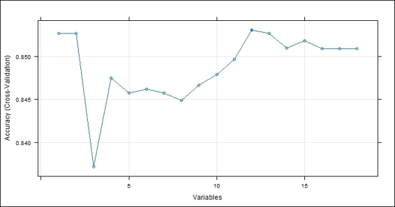
Figure 3: The feature selection result
10.We can then examine the best subset of the variables:
11.> ldaProfile$optVariables
12. [1] "total_day_charge"
13. [2] "total_day_minutes"
14. [3] "intl_no"
15. [4] "number_customer_service_calls"
16. [5] "total_eve_charge"
17. [6] "total_eve_minutes"
18. [7] "voidce_yes"
19. [8] "total_intl_calls"
20. [9] "number_vmail_messages"
21.[10] "total_intl_charge"
22.[11] "total_intl_minutes"
23.[12] "total_night_minutes"
11.Now, we can examine the fitted model:
12.> ldaProfile$fit
13.Call:
14.lda(x, y)
15.
16.Prior probabilities of groups:
17. yes no
18.0.1477322 0.8522678
19.
20.Group means:
21. total_day_charge total_day_minutes intl_no
22.yes 35.00143 205.8877 0.7046784
23.no 29.62402 174.2555 0.9351242
24. number_customer_service_calls total_eve_charge
25.yes 2.204678 18.16702
26.no 1.441460 16.96789
27. total_eve_minutes voidce_yes total_intl_calls
28.yes 213.7269 0.1666667 4.134503
29.no 199.6197 0.2954891 4.514445
30. number_vmail_messages total_intl_charge
31.yes 5.099415 2.899386
32.no 8.674607 2.741343
33. total_intl_minutes total_night_minutes
34.yes 10.73684 205.4640
35.no 10.15119 201.4184
36.
37.Coefficients of linear discriminants:
38. LD1
39.total_day_charge 0.715025524
40.total_day_minutes -0.130486470
41.intl_no 2.259889324
42.number_customer_service_calls -0.421997335
43.total_eve_charge -2.390372793
44.total_eve_minutes 0.198406977
45.voidce_yes 0.660927935
46.total_intl_calls 0.066240268
47.number_vmail_messages -0.003529233
48.total_intl_charge 2.315069869
49.total_intl_minutes -0.693504606
50.total_night_minutes -0.002127471
12.Finally, we can calculate the performance across resamples:
13.> postResample(predict(ldaProfile, testset[, !names(testset) %in% c("churn")]), testset[,c("churn")])
14.Accuracy Kappa
15.0.8605108 0.2672027
How it works...
In this recipe, we perform feature selection using the caret package. As there are factor-coded attributes within the dataset, we first use a function called model.matrix to transform the factor-coded attributes into multiple binary attributes. Therefore, we transform the international_plan attribute to intl_yes and intl_no. Additionally, we transform the voice_mail_plan attribute to voice_yes and voice_no.
Next, we set up control parameters for training using the cross-validation method, cv, with the linear discriminant function, ldaFuncs. Then, we use the recursive feature elimination, rfe, to perform feature selection with the use of the control function, ldaFuncs. The rfe function generates the summary of feature selection, which contains resampling a performance over the subset size and top variables.
We can then use the obtained model information to plot the number of variables against accuracy. From Figure 3, it is obvious that using 12 features can obtain the best accuracy. In addition to this, we can retrieve the best subset of the variables in (12 variables in total) the fitted model. Lastly, we can calculate the performance across resamples, which yields an accuracy of 0.86 and a kappa of 0.27.
See also
· In order to specify the algorithm used to control feature selection, one can change the control function specified in rfeControl. Here are some of the options you can use:
· caretFuncs SVM (caret)
· lmFuncs lm (base)
· rfFuncs RF(randomForest)
· treebagFuncs DT (ipred)
· ldaFuncs lda(base)
· nbFuncs NB(klaR)
· gamFuncs gam(gam)
Measuring the performance of the regression model
To measure the performance of a regression model, we can calculate the distance from predicted output and the actual output as a quantifier of the performance of the model. Here, we often use the root mean square error (RMSE), relative square error (RSE) and R-Square as common measurements. In the following recipe, we will illustrate how to compute these measurements from a built regression model.
Getting ready
In this recipe, we will use the Quartet dataset, which contains four regression datasets, as our input data source.
How to do it...
Perform the following steps to measure the performance of the regression model:
1. Load the Quartet dataset from the car package:
2. > library(car)
3. > data(Quartet)
2. Plot the attribute, y3, against x using the lm function:
3. > plot(Quartet$x, Quartet$y3)
4. > lmfit = lm(Quartet$y3~Quartet$x)
5. > abline(lmfit, col="red")
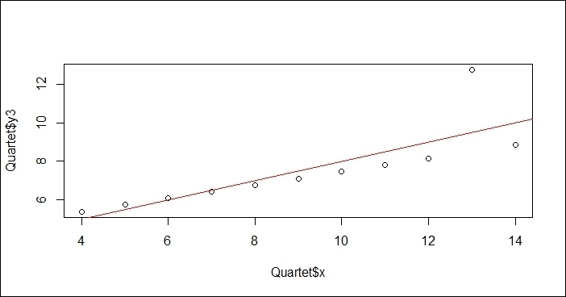
Figure 4: The linear regression plot
3. You can retrieve predicted values by using the predict function:
4. > predicted= predict(lmfit, newdata=Quartet[c("x")])
4. Now, you can calculate the root mean square error:
5. > actual = Quartet$y3
6. > rmse = (mean((predicted - actual)^2))^0.5
7. > rmse
8. [1] 1.118286
5. You can calculate the relative square error:
6. > mu = mean(actual)
7. > rse = mean((predicted - actual)^2) / mean((mu - actual)^2)
8. > rse
9. [1] 0.333676
6. Also, you can use R-Square as a measurement:
7. > rsquare = 1 - rse
8. > rsquare
9. [1] 0.666324
7. Then, you can plot attribute, y3, against x using the rlm function from the MASS package:
8. > library(MASS)
9. > plot(Quartet$x, Quartet$y3)
10.> rlmfit = rlm(Quartet$y3~Quartet$x)
11.> abline(rlmfit, col="red")
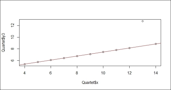
Figure 5: The robust linear regression plot on the Quartet dataset
8. You can then retrieve the predicted value using the predict function:
9. > predicted = predict(rlmfit, newdata=Quartet[c("x")])
9. Next, you can calculate the root mean square error using the distance of the predicted and actual value:
10.> actual = Quartet$y3
11.> rmse = (mean((predicted - actual)^2))^0.5
12.> rmse
13.[1] 1.279045
10.Calculate the relative square error between the predicted and actual labels:
11.> mu = mean(actual)
12.> rse =mean((predicted - actual)^2) / mean((mu - actual)^2)
13.> rse
14.[1] 0.4365067
11.Now, you can calculate the R-Square value:
12.> rsquare = 1 - rse
13.> rsquare
14.[1] 0.5634933
How it works...
The measurement of the performance of the regression model employs the distance between the predicted value and the actual value. We often use these three measurements, root mean square error, relative square error, and R-Square, as the quantifier of the performance of regression models. In this recipe, we first load the Quartet data from the car package. We then use the lm function to fit the linear model, and add the regression line on a scatter plot of the x variable against the y3 variable. Next, we compute the predicted value using the predict function, and begin to compute the root mean square error (RMSE), relative square error (RSE), and R-Square for the built model.
As this dataset has an outlier at x=13, we would like to quantify how the outlier affects the performance measurement. To achieve this, we first train a regression model using the rlm function from the MASS package. Similar to the previous step, we then generate a performance measurement of the root square mean error, relative error and R-Square. From the output measurement, it is obvious that the mean square error and the relative square errors of the lmmodel are smaller than the model built by rlm, and the score of R-Square shows that the model built with lm has a greater prediction power. However, for the actual scenario, we should remove the outlier at x=13. This comparison shows that the outlier may be biased toward the performance measure and may lead us to choose the wrong model.
There's more…
If you would like to perform cross-validation on a linear regression model, you can use the tune function within the e1071 package:
> tune(lm, y3~x, data = Quartet)
Error estimation of 'lm' using 10-fold cross validation: 2.33754
Other than the e1071 package, you can use the train function from the caret package to perform cross-validation. In addition to this, you can also use cv.lm from the DAAG package to achieve the same goal.
Measuring prediction performance with a confusion matrix
To measure the performance of a classification model, we can first generate a classification table based on our predicted label and actual label. Then, we can use a confusion matrix to obtain performance measures such as precision, recall, specificity, and accuracy. In this recipe, we will demonstrate how to retrieve a confusion matrix using the caret package.
Getting ready
In this recipe, we will continue to use the telecom churn dataset as our example dataset.
How to do it...
Perform the following steps to generate a classification measurement:
1. Train an svm model using the training dataset:
2. > svm.model= train(churn ~ .,
3. + data = trainset,
4. + method = "svmRadial")
2. You can then predict labels using the fitted model, svm.model:
3. > svm.pred = predict(svm.model, testset[,! names(testset) %in% c("churn")])
3. Next, you can generate a classification table:
4. > table(svm.pred, testset[,c("churn")])
5.
6. svm.pred yes no
7. yes 73 16
8. no 68 861
4. Lastly, you can generate a confusion matrix using the prediction results and the actual labels from the testing dataset:
5. > confusionMatrix(svm.pred, testset[,c("churn")])
6. Confusion Matrix and Statistics
7.
8. Reference
9. Prediction yes no
10. yes 73 16
11. no 68 861
12.
13. Accuracy : 0.9175
14. 95% CI : (0.8989, 0.9337)
15. No Information Rate : 0.8615
16. P-Value [Acc > NIR] : 2.273e-08
17.
18. Kappa : 0.5909
19. Mcnemar's Test P-Value : 2.628e-08
20.
21. Sensitivity : 0.51773
22. Specificity : 0.98176
23. Pos Pred Value : 0.82022
24. Neg Pred Value : 0.92680
25. Prevalence : 0.13851
26. Detection Rate : 0.07171
27. Detection Prevalence : 0.08743
28. Balanced Accuracy : 0.74974
29.
30. 'Positive' Class : yes
How it works...
In this recipe, we demonstrate how to obtain a confusion matrix to measure the performance of a classification model. First, we use the train function from the caret package to train an svm model. Next, we use the predict function to extract the predicted labels of the svm model using the testing dataset. Then, we perform the table function to obtain the classification table based on the predicted and actual labels. Finally, we use the confusionMatrix function from the caret package to a generate a confusion matrix to measure the performance of the classification model.
See also
· If you are interested in the available methods that can be used in the train function, you can refer to this website: http://topepo.github.io/caret/modelList.html
Measuring prediction performance using ROCR
A receiver operating characteristic (ROC) curve is a plot that illustrates the performance of a binary classifier system, and plots the true positive rate against the false positive rate for different cut points. We most commonly use this plot to calculate the area under curve (AUC) to measure the performance of a classification model. In this recipe, we will demonstrate how to illustrate an ROC curve and calculate the AUC to measure the performance of a classification model.
Getting ready
In this recipe, we will continue using the telecom churn dataset as our example dataset.
How to do it...
Perform the following steps to generate two different classification examples with different costs:
1. First, you should install and load the ROCR package:
2. > install.packages("ROCR")
3. > library(ROCR)
2. Train the svm model using the training dataset with a probability equal to TRUE:
3. > svmfit=svm(churn~ ., data=trainset, prob=TRUE)
3. Make predictions based on the trained model on the testing dataset with the probability set as TRUE:
4. >pred=predict(svmfit,testset[, !names(testset) %in% c("churn")], probability=TRUE)
4. Obtain the probability of labels with yes:
5. > pred.prob = attr(pred, "probabilities")
6. > pred.to.roc = pred.prob[, 2]
5. Use the prediction function to generate a prediction result:
6. > pred.rocr = prediction(pred.to.roc, testset$churn)
6. Use the performance function to obtain the performance measurement:
7. > perf.rocr = performance(pred.rocr, measure = "auc", x.measure = "cutoff")
8. > perf.tpr.rocr = performance(pred.rocr, "tpr","fpr")
7. Visualize the ROC curve using the plot function:
8. > plot(perf.tpr.rocr, colorize=T,main=paste("AUC:",(perf.rocr@y.values)))
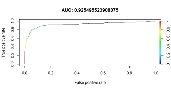
Figure 6: The ROC curve for the svm classifier performance
How it works...
In this recipe, we demonstrated how to generate an ROC curve to illustrate the performance of a binary classifier. First, we should install and load the library, ROCR. Then, we use svm, from the e1071 package, to train a classification model, and then use the model to predict labels for the testing dataset. Next, we use the prediction function (from the package, ROCR) to generate prediction results. We then adapt the performance function to obtain the performance measurement of the true positive rate against the false positive rate. Finally, we use the plot function to visualize the ROC plot, and add the value of AUC on the title. In this example, the AUC value is 0.92, which indicates that the svm classifier performs well in classifying telecom user churn datasets.
See also
· For those interested in the concept and terminology of ROC, you can refer to http://en.wikipedia.org/wiki/Receiver_operating_characteristic
Comparing an ROC curve using the caret package
In previous chapters, we introduced many classification methods; each method has its own advantages and disadvantages. However, when it comes to the problem of how to choose the best fitted model, you need to compare all the performance measures generated from different prediction models. To make the comparison easy, the caret package allows us to generate and compare the performance of models. In this recipe, we will use the function provided by the caret package to compare different algorithm trained models on the same dataset.
Getting ready
Here, we will continue to use telecom dataset as our input data source.
How to do it...
Perform the following steps to generate an ROC curve of each fitted model:
1. Install and load the library, pROC:
2. > install.packages("pROC")
3. > library("pROC")
2. Set up the training control with a 10-fold cross-validation in 3 repetitions:
3. > control = trainControl(method = "repeatedcv",
4. + number = 10,
5. + repeats = 3,
6. + classProbs = TRUE,
7. + summaryFunction = twoClassSummary)
3. Then, you can train a classifier on the training dataset using glm:
4. > glm.model= train(churn ~ .,
5. + data = trainset,
6. + method = "glm",
7. + metric = "ROC",
8. + trControl = control)
4. Also, you can train a classifier on the training dataset using svm:
5. > svm.model= train(churn ~ .,
6. + data = trainset,
7. + method = "svmRadial",
8. + metric = "ROC",
9. + trControl = control)
5. To see how rpart performs on the training data, we use the rpart function:
6. > rpart.model= train(churn ~ .,
7. + data = trainset,
8. + method = "rpart",
9. + metric = "ROC",
10.+ trControl = control)
6. You can make predictions separately based on different trained models:
7. > glm.probs = predict(glm.model, testset[,! names(testset) %in% c("churn")], type = "prob")
8. > svm.probs = predict(svm.model, testset[,! names(testset) %in% c("churn")], type = "prob")
9. > rpart.probs = predict(rpart.model, testset[,! names(testset) %in% c("churn")], type = "prob")
7. You can generate the ROC curve of each model, and plot the curve on the same figure:
8. > glm.ROC = roc(response = testset[,c("churn")],
9. + predictor =glm.probs$yes,
10.+ levels = levels(testset[,c("churn")]))
11.> plot(glm.ROC, type="S", col="red")
12.
13.Call:
14.roc.default(response = testset[, c("churn")], predictor = glm.probs$yes, levels = levels(testset[, c("churn")]))
15.
16.Data: glm.probs$yes in 141 controls (testset[, c("churn")] yes) > 877 cases (testset[, c("churn")] no).
17.Area under the curve: 0.82
18.
19.> svm.ROC = roc(response = testset[,c("churn")],
20.+ predictor =svm.probs$yes,
21.+ levels = levels(testset[,c("churn")]))
22.> plot(svm.ROC, add=TRUE, col="green")
23.
24.Call:
25.roc.default(response = testset[, c("churn")], predictor = svm.probs$yes, levels = levels(testset[, c("churn")]))
26.
27.Data: svm.probs$yes in 141 controls (testset[, c("churn")] yes) > 877 cases (testset[, c("churn")] no).
28.Area under the curve: 0.9233
29.
30.> rpart.ROC = roc(response = testset[,c("churn")],
31.+ predictor =rpart.probs$yes,
32.+ levels = levels(testset[,c("churn")]))
33.> plot(rpart.ROC, add=TRUE, col="blue")
34.
35.Call:
36.roc.default(response = testset[, c("churn")], predictor = rpart.probs$yes, levels = levels(testset[, c("churn")]))
37.
38.Data: rpart.probs$yes in 141 controls (testset[, c("churn")] yes) > 877 cases (testset[, c("churn")] no).
39.Area under the curve: 0.7581
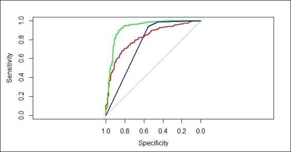
Figure 7: The ROC curve for the performance of three classifiers
How it works...
Here, we demonstrate how we can compare fitted models by illustrating their ROC curve in one figure. First, we set up the control of the training process with a 10-fold cross validation in 3 repetitions with the performance evaluation in twoClassSummary. After setting up control of the training process, we then apply glm, svm, and rpart algorithms on the training dataset to fit the classification models. Next, we can make a prediction based on each generated model and plot the ROC curve, respectively. Within the generated figure, we find that the model trained by svm has the largest area under curve, which is 0.9233 (plotted in green), the AUC of the glm model (red) is 0.82, and the AUC of the rpart model (blue) is 0.7581. From Figure 7, it is obvious that svm performs the best among all the fitted models on this training dataset (without requiring tuning).
See also
· We use another ROC visualization package, pROC, which can be employed to display and analyze ROC curves. If you would like to know more about the package, please use the help function:
· > help(package="pROC")
Measuring performance differences between models with the caret package
In the previous recipe, we introduced how to generate ROC curves for each generated model, and have the curve plotted on the same figure. Apart from using an ROC curve, one can use the resampling method to generate statistics of each fitted model in ROC, sensitivity and specificity metrics. Therefore, we can use these statistics to compare the performance differences between each model. In the following recipe, we will introduce how to measure performance differences between fitted models with the caret package.
Getting ready
One needs to have completed the previous recipe by storing the glm fitted model, svm fitted model, and the rpart fitted model into glm.model, svm.model, and rpart.model, respectively.
How to do it...
Perform the following steps to measure performance differences between each fitted model:
1. Resample the three generated models:
2. > cv.values = resamples(list(glm = glm.model, svm=svm.model, rpart = rpart.model))
2. Then, you can obtain a summary of the resampling result:
3. > summary(cv.values)
4.
5. Call:
6. summary.resamples(object = cv.values)
7.
8. Models: glm, svm, rpart
9. Number of resamples: 30
10.
11.ROC
12. Min. 1st Qu. Median Mean 3rd Qu. Max. NA's
13.glm 0.7206 0.7847 0.8126 0.8116 0.8371 0.8877 0
14.svm 0.8337 0.8673 0.8946 0.8929 0.9194 0.9458 0
15.rpart 0.2802 0.7159 0.7413 0.6769 0.8105 0.8821 0
16.
17.Sens
18. Min. 1st Qu. Median Mean 3rd Qu. Max. NA's
19.glm 0.08824 0.2000 0.2286 0.2194 0.2517 0.3529 0
20.svm 0.44120 0.5368 0.5714 0.5866 0.6424 0.7143 0
21.rpart 0.20590 0.3742 0.4706 0.4745 0.5929 0.6471 0
22.
23.Spec
24. Min. 1st Qu. Median Mean 3rd Qu. Max. NA's
25.glm 0.9442 0.9608 0.9746 0.9701 0.9797 0.9949 0
26.svm 0.9442 0.9646 0.9746 0.9740 0.9835 0.9949 0
27.rpart 0.9492 0.9709 0.9797 0.9780 0.9848 0.9949 0
3. Use dotplot to plot the resampling result in the ROC metric:
4. > dotplot(cv.values, metric = "ROC")
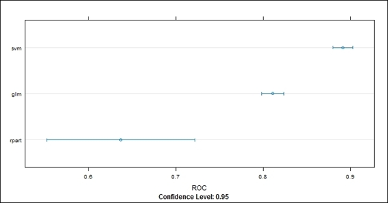
Figure 8: The dotplot of resampling result in ROC metric
4. Also, you can use a box-whisker plot to plot the resampling result:
5. > bwplot(cv.values, layout = c(3, 1))
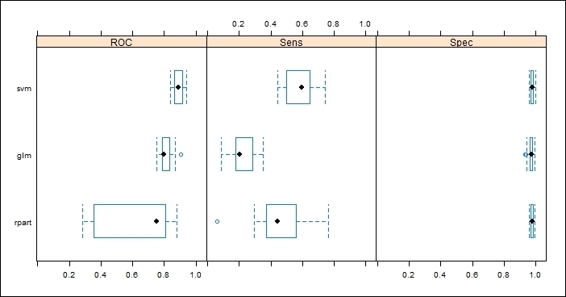
Figure 9: The box-whisker plot of resampling result
How it works...
In this recipe, we demonstrate how to measure the performance differences among three fitted models using the resampling method. First, we use the resample function to generate the statistics of each fitted model (svm.model, glm.model, and rpart.model). Then, we can use the summary function to obtain the statistics of these three models in the ROC, sensitivity and specificity metrics. Next, we can apply a dotplot on the resampling result to see how ROC varied between each model. Last, we use a box-whisker plot on the resampling results to show the box-whisker plot of different models in the ROC, sensitivity and specificity metrics on a single plot.
See also
· Besides using dotplot and bwplot to measure performance differences, one can use densityplot, splom, and xyplot to visualize the performance differences of each fitted model in the ROC, sensitivity, and specificity metrics.
All materials on the site are licensed Creative Commons Attribution-Sharealike 3.0 Unported CC BY-SA 3.0 & GNU Free Documentation License (GFDL)
If you are the copyright holder of any material contained on our site and intend to remove it, please contact our site administrator for approval.
© 2016-2026 All site design rights belong to S.Y.A.