Machine Learning with R Cookbook (2015)

Chapter 8. Ensemble Learning

In this chapter, we will cover the following topics:

· Classifying data with the bagging method

· Performing cross-validation with the bagging method

· Classifying data with the boosting method

· Performing cross-validation with the boosting method

· Classifying data with gradient boosting

· Calculating the margins of a classifier

· Calculating the error evolution of the ensemble method

· Classifying the data with random forest

· Estimating the prediction errors of different classifiers

Introduction

Ensemble learning is a method to combine results produced by different learners into one format, with the aim of producing better classification results and regression results. In previous chapters, we discussed several classification methods. These methods take different approaches but they all have the same goal, that is, finding an optimum classification model. However, a single classifier may be imperfect, which may misclassify data in certain categories. As not all classifiers are imperfect, a better approach is to average the results by voting. In other words, if we average the prediction results of every classifier with the same input, we may create a superior model compared to using anindividual method.

In ensemble learning, bagging, boosting, and random forest are the three most common methods:

· Bagging is a voting method, which first uses Bootstrap to generate a different training set, and then uses the training set to make different base learners. The bagging method employs a combination of base learners to make a better prediction.

· Boosting is similar to the bagging method. However, what makes boosting different is that it first constructs the base learning in sequence, where each successive learner is built for the prediction residuals of the preceding learner. With the means to create a complementary learner, it uses the mistakes made by previous learners to train the next base learner.

· Random forest uses the classification results voted from many classification trees. The idea is simple; a single classification tree will obtain a single classification result with a single input vector. However, a random forest grows many classification trees, obtaining multiple results from a single input. Therefore, a random forest will use the majority of votes from all the decision trees to classify data or use an average output for regression.

In the following recipes, we will discuss how to use bagging and boosting to classify data. We can then perform cross-validation to estimate the error rate of each classifier. In addition to this, we'll introduce the use of a margin to measure the certainty of a model. Next, we cover random forests, similar to the bagging and boosting methods, and introduce how to train the model to classify data and use margins to estimate the model certainty. Lastly, we'll demonstrate how to estimate the error rate of each classifier, and use the error rate to compare the performance of different classifiers.

Classifying data with the bagging method

The adabag package implements both boosting and bagging methods. For the bagging method, the package implements Breiman's Bagging algorithm, which first generates multiple versions of classifiers, and then obtains an aggregated classifier. In this recipe, we will illustrate how to use the bagging method from adabag to generate a classification model using the telecom churn dataset.

Getting ready

In this recipe, we continue to use the telecom churn dataset as the input data source for the bagging method. For those who have not prepared the dataset, please refer to Chapter 5, Classification (I) – Tree, Lazy, and Probabilistic, for detailed information.

How to do it...

Perform the following steps to generate a classification model for the telecom churn dataset:

1. First, you need to install and load the adabag package (it might take a while to install adabag):

2. > install.packages("adabag")

3. > library(adabag)

2. Next, you can use the bagging function to train a training dataset (the result may vary during the training process):

3. > set.seed(2)

4. > churn.bagging = bagging(churn ~ ., data=trainset, mfinal=10)

3. Access the variable importance from the bagging result:

4. > churn.bagging$importance

5. international_plan number_customer_service_calls

6. 10.4948380 16.4260510

7. number_vmail_messages total_day_calls

8. 0.5319143 0.3774190

9. total_day_charge total_day_minutes

10. 0.0000000 28.7545042

11. total_eve_calls total_eve_charge

12. 0.1463585 0.0000000

13. total_eve_minutes total_intl_calls

14. 14.2366754 8.7733895

15. total_intl_charge total_intl_minutes

16. 0.0000000 9.7838256

17. total_night_calls total_night_charge

18. 0.4349952 0.0000000

19. total_night_minutes voice_mail_plan

20. 2.3379622 7.7020671

4. After generating the classification model, you can use the predicted results from the testing dataset:

5. > churn.predbagging= predict.bagging(churn.bagging, newdata=testset)

5. From the predicted results, you can obtain a classification table:

6. > churn.predbagging$confusion

7. Observed Class

8. Predicted Class yes no

9. no 35 866

10. yes 106 11

6. Finally, you can retrieve the average error of the bagging result:

7. > churn.predbagging$error

8. [1] 0.0451866

How it works...

Bagging is derived from the name Bootstrap aggregating, which is a stable, accurate, and easy to implement model for data classification and regression. The definition of bagging is as follows: given a training dataset of size n, bagging performs Bootstrap sampling and generates m new training sets, Di, each of size n. Finally, we can fit m Bootstrap samples to m models and combine the result by averaging the output (for regression) or voting (for classification):

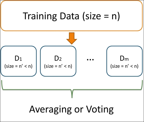
An illustration of bagging method

The advantage of using bagging is that it is a powerful learning method, which is easy to understand and implement. However, the main drawback of this technique is that it is hard to analyze the result.

In this recipe, we use the boosting method from adabag to classify the telecom churn data. Similar to other classification methods discussed in previous chapters, you can train a boosting classifier with a formula and a training dataset. Additionally, you can set the number of iterations to 10 in the mfinal argument. Once the classification model is built, you can examine the importance of each attribute. Ranking the attributes by importance reveals that the number of customer service calls play a crucial role in the classification model.

Next, with a fitted model, you can apply the predict.bagging function to predict the labels of the testing dataset. Therefore, you can use the labels of the testing dataset and predicted results to generate a classification table and obtain the average error, which is 0.045 in this example.

There's more...

Besides adabag, the ipred package provides a bagging method for a classification tree. We demonstrate here how to use the bagging method of the ipred package to train a classification model:

1. First, you need to install and load the ipred package:

2. > install.packages("ipred")

3. > library(ipred)

2. You can then use the bagging method to fit the classification method:

3. > churn.bagging = bagging(churn ~ ., data = trainset, coob = T)

4. > churn.bagging

6. Bagging classification trees with 25 bootstrap replications

8. Call: bagging.data.frame(formula = churn ~ ., data = trainset, coob = T)

10.Out-of-bag estimate of misclassification error: 0.0605

3. Obtain an out of bag estimate of misclassification of the errors:

4. > mean(predict(churn.bagging) != trainset$churn)

5. [1] 0.06047516

4. You can then use the predict function to obtain the predicted labels of the testing dataset:

5. > churn.prediction = predict(churn.bagging, newdata=testset, type="class")

5. Obtain the classification table from the labels of the testing dataset and prediction result:

6. > prediction.table = table(churn.prediction, testset$churn)

8. churn.prediction yes no

9. no 31 869

10. yes 110 8

Performing cross-validation with the bagging method

To assess the prediction power of a classifier, you can run a cross-validation method to test the robustness of the classification model. In this recipe, we will introduce how to use bagging.cv to perform cross-validation with the bagging method.

Getting ready

In this recipe, we continue to use the telecom churn dataset as the input data source to perform a k-fold cross-validation with the bagging method.

How to do it...

Perform the following steps to retrieve the minimum estimation errors by performing cross-validation with the bagging method:

1. First, we use bagging.cv to make a 10-fold classification on the training dataset with 10 iterations:

2. > churn.baggingcv = bagging.cv(churn ~ ., v=10, data=trainset, mfinal=10)

2. You can then obtain the confusion matrix from the cross-validation results:

3. > churn.baggingcv$confusion

4. Observed Class

5. Predicted Class yes no

6. no 100 1938

7. yes 242 35

3. Lastly, you can retrieve the minimum estimation errors from the cross-validation results:

4. > churn.baggingcv$error

5. [1] 0.05831533

How it works...

The adabag package provides a function to perform the k-fold validation with either the bagging or boosting method. In this example, we use bagging.cv to make the k-fold cross-validation with the bagging method. We first perform a 10-fold cross validation with 10 iterations by specifying v=10 and mfinal=10. Please note that this is quite time consuming due to the number of iterations. After the cross-validation process is complete, we can obtain the confusion matrix and average errors (0.058 in this case) from the cross-validation results.

See also

· For those interested in tuning the parameters of bagging.cv, please view the bagging.cv document by using the help function:

· > help(bagging.cv)

Classifying data with the boosting method

Similar to the bagging method, boosting starts with a simple or weak classifier and gradually improves it by reweighting the misclassified samples. Thus, the new classifier can learn from previous classifiers. The adabag package provides implementation of the AdaBoost.M1 and SAMME algorithms. Therefore, one can use the boosting method in adabag to perform ensemble learning. In this recipe, we will use the boosting method in adabag to classify the telecom churn dataset.

Getting ready

In this recipe, we will continue to use the telecom churn dataset as the input data source to perform classifications with the boosting method. Also, you need to have the adabag package loaded in R before commencing the recipe.

How to do it...

Perform the following steps to classify the telecom churn dataset with the boosting method:

1. You can use the boosting function from the adabag package to train the classification model:

2. > set.seed(2)

3. > churn.boost = boosting(churn ~.,data=trainset,mfinal=10, coeflearn="Freund", boos=FALSE , control=rpart.control(maxdepth=3))

2. You can then make a prediction based on the boosted model and testing dataset:

3. > churn.boost.pred = predict.boosting(churn.boost,newdata=testset)

3. Next, you can retrieve the classification table from the predicted results:

4. > churn.boost.pred$confusion

5. Observed Class

6. Predicted Class yes no

7. no 41 858

8. yes 100 19

4. Finally, you can obtain the average errors from the predicted results:

5. > churn.boost.pred$error

6. [1] 0.0589391

How it works...

The idea of boosting is to "boost" weak learners (for example, a single decision tree) into strong learners. Assuming that we have n points in our training dataset, we can assign a weight, Wi (0 <= i <n), for each point. Then, during the iterative learning process (we assume the number of iterations is m), we can reweigh each point in accordance with the classification result in each iteration. If the point is correctly classified, we should decrease the weight. Otherwise, we increase the weight of the point. When the iteration process is finished, we can then obtain the m fitted model, f_i(x) (0 <= i <n). Finally, we can obtain the final prediction through the weighted average of each tree's prediction, where the weight, b, is based on the quality of each tree:

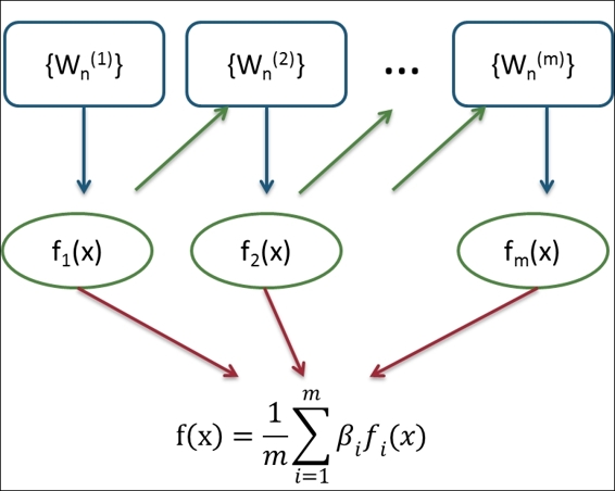
An illustration of boosting method

Both bagging and boosting are ensemble methods, which combine the prediction power of each single learner into a strong learner. The difference between bagging and boosting is that the bagging method combines independent models, but boosting performs an iterative process to reduce the errors of preceding models by predicting them with successive models.

In this recipe, we demonstrate how to fit a classification model within the boosting method. Similar to bagging, one has to specify the formula and the training dataset used to train the classification model. In addition, one can specify parameters, such as the number of iterations (mfinal), the weight update coefficient (coeflearn), the weight of how each observation is used (boos), and the control for rpart (a single decision tree). In this recipe, we set the iteration to 10, using Freund (the AdaBoost.M1 algorithm implemented method) as coeflearn, boos set to false and max depth set to 3 for rpart configuration.

We use the boosting method to fit the classification model and then save it in churn.boost. We can then obtain predicted labels using the prediction function. Furthermore, we can use the table function to retrieve a classification table based on the predicted labels and testing the dataset labels. Lastly, we can get the average errors of the predicted results.

There's more...

In addition to using the boosting function in the adabag package, one can also use the caret package to perform a classification with the boosting method:

1. First, load the mboost and pROC package:

2. > library(mboost)

3. > install.packages("pROC")

4. > library(pROC)

2. We can then set the training control with the trainControl function and use the train function to train the classification model with adaboost:

3. > set.seed(2)

4. > ctrl = trainControl(method = "repeatedcv", repeats = 1, classProbs = TRUE, summaryFunction = twoClassSummary)

5. > ada.train = train(churn ~ ., data = trainset, method = "ada", metric = "ROC", trControl = ctrl)

3. Use the summary function to obtain the details of the classification model:

4. > ada.train$result

5. nu maxdepth iter ROC Sens Spec ROCSD SensSD SpecSD

6. 1 0.1 1 50 0.8571988 0.9152941 0.012662155 0.03448418 0.04430519 0.007251045

7. 4 0.1 2 50 0.8905514 0.7138655 0.006083679 0.03538445 0.10089887 0.006236741

8. 7 0.1 3 50 0.9056456 0.4036134 0.007093780 0.03934631 0.09406015 0.006407402

9. 2 0.1 1 100 0.8550789 0.8918487 0.015705276 0.03434382 0.06190546 0.006503191

10.5 0.1 2 100 0.8907720 0.6609244 0.009626724 0.03788941 0.11403364 0.006940001

11.8 0.1 3 100 0.9077750 0.3832773 0.005576065 0.03601187 0.09630026 0.003738978

12.3 0.1 1 150 0.8571743 0.8714286 0.016720505 0.03481526 0.06198773 0.006767313

13.6 0.1 2 150 0.8929524 0.6171429 0.011654617 0.03638272 0.11383803 0.006777465

14.9 0.1 3 150 0.9093921 0.3743697 0.007093780 0.03258220 0.09504202 0.005446136

4. Use the plot function to plot the ROC curve within different iterations:

5. > plot(ada.train)

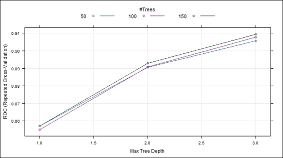
The repeated cross validation plot

5. Finally, we can make predictions using the predict function and view the classification table:

6. > ada.predict = predict(ada.train, testset, "prob")

7. > ada.predict.result = ifelse(ada.predict[1] > 0.5, "yes", "no")

9. > table(testset$churn, ada.predict.result)

10. ada.predict.result

11. no yes

12. yes 40 101

13. no 872 5

Performing cross-validation with the boosting method

Similar to the bagging function, adabag provides a cross-validation function for the boosting method, named boosting.cv. In this recipe, we will demonstrate how to perform cross-validation using boosting.cv from the package, adabag.

Getting ready

In this recipe, we continue to use the telecom churn dataset as the input data source to perform a k-fold cross-validation with the boosting method.

How to do it...

Perform the following steps to retrieve the minimum estimation errors via cross-validation with the boosting method:

1. First, you can use boosting.cv to cross-validate the training dataset:

2. > churn.boostcv = boosting.cv(churn ~ ., v=10, data=trainset, mfinal=5,control=rpart.control(cp=0.01))

2. You can then obtain the confusion matrix from the boosting results:

3. > churn.boostcv$confusion

4. Observed Class

5. Predicted Class yes no

6. no 119 1940

7. yes 223 33

3. Finally, you can retrieve the average errors of the boosting method:

4. > churn.boostcv$error

5. [1] 0.06565875

How it works...

Similar to bagging.cv, we can perform cross-validation with the boosting method using boosting.cv. If v is set to 10 and mfinal is set to 5, the boosting method will perform 10-fold cross-validations with five iterations. Also, one can set the control of the rpart fit within the parameter. We can set the complexity parameter to 0.01 in this example. Once the training is complete, the confusion matrix and average errors of the boosted results will be obtained.

See also

· For those who require more information on tuning the parameters of boosting.cv, please view the boosting.cv document by using the help function:

· > help(boosting.cv)

Classifying data with gradient boosting

Gradient boosting ensembles weak learners and creates a new base learner that maximally correlates with the negative gradient of the loss function. One may apply this method on either regression or classification problems, and it will perform well in different datasets. In this recipe, we will introduce how to use gbm to classify a telecom churn dataset.

Getting ready

How to do it...

Perform the following steps to calculate and classify data with the gradient boosting method:

1. First, install and load the package, gbm:

2. > install.packages("gbm")

3. > library(gbm)

2. The gbm function only uses responses ranging from 0 to 1; therefore, you should transform yes/no responses to numeric responses (0/1):

3. > trainset$churn = ifelse(trainset$churn == "yes", 1, 0)

3. Next, you can use the gbm function to train a training dataset:

4. > set.seed(2)

5. > churn.gbm = gbm(formula = churn ~ .,distribution = "bernoulli",data = trainset,n.trees = 1000,interaction.depth = 7,shrinkage = 0.01, cv.folds=3)

4. Then, you can obtain the summary information from the fitted model:

5. > summary(churn.gbm)

6. var rel.inf

7. total_day_minutes total_day_minutes 28.1217147

8. total_eve_minutes total_eve_minutes 16.8097151

9. number_customer_service_calls number_customer_service_calls 12.7894464

10.total_intl_minutes total_intl_minutes 9.4515822

11.total_intl_calls total_intl_calls 8.1379826

12.international_plan international_plan 8.0703900

13.total_night_minutes total_night_minutes 4.0805153

14.number_vmail_messages number_vmail_messages 3.9173515

15.voice_mail_plan voice_mail_plan 2.5501480

16.total_night_calls total_night_calls 2.1357970

17.total_day_calls total_day_calls 1.7367888

18.total_eve_calls total_eve_calls 1.4398047

19.total_eve_charge total_eve_charge 0.5457486

20.total_night_charge total_night_charge 0.2130152

21.total_day_charge total_day_charge 0.0000000

22.total_intl_charge total_intl_charge 0.0000000

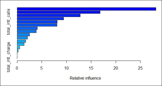
Relative influence plot of fitted model

5. You can obtain the best iteration using cross-validation:

6. > churn.iter = gbm.perf(churn.gbm,method="cv")

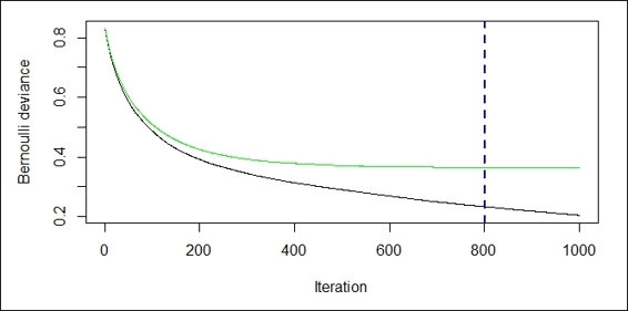
The performance measurement plot

6. Then, you can retrieve the odd value of the log returned from the Bernoulli loss function:

7. > churn.predict = predict(churn.gbm, testset, n.trees = churn.iter)

8. > str(churn.predict)

9. num [1:1018] -3.31 -2.91 -3.16 -3.47 -3.48 ...

7. Next, you can plot the ROC curve and get the best cut off that will have the maximum accuracy:

8. > churn.roc = roc(testset$churn, churn.predict)

9. > plot(churn.roc)

10.Call:

11.roc.default(response = testset$churn, predictor = churn.predict)

12.Data: churn.predict in 141 controls (testset$churn yes) > 877 cases (testset$churn no).

13.Area under the curve: 0.9393

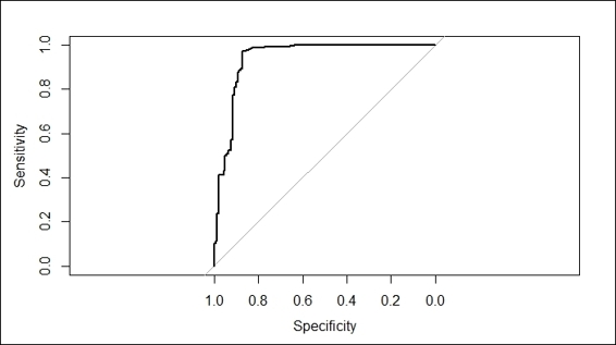
The ROC curve of fitted model

8. You can retrieve the best cut off with the coords function and use this cut off to obtain the predicted label:

9. > coords(churn.roc, "best")

10. threshold specificity sensitivity

11. -0.9495258 0.8723404 0.9703535

12.> churn.predict.class = ifelse(churn.predict > coords(churn.roc, "best")["threshold"], "yes", "no")

9. Lastly, you can obtain the classification table from the predicted results:

10.> table( testset$churn,churn.predict.class)

11. churn.predict.class

12. no yes

13. yes 18 123

14. no 851 26

How it works...

The algorithm of gradient boosting involves, first, the process computes the deviation of residuals for each partition, and then, determines the best data partitioning in each stage. Next, the successive model will fit the residuals from the previous stage and build a new model to reduce the residual variance (an error). The reduction of the residual variance follows the functional gradient descent technique, in which it minimizes the residual variance by going down its derivative, as show here:

Gradient descent method

In this recipe, we use the gradient boosting method from gbm to classify the telecom churn dataset. To begin the classification, we first install and load the gbm package. Then, we use the gbm function to train the classification model. Here, as our prediction target is the churn attribute, which is a binary outcome, we therefore set the distribution as bernoulli in the distribution argument. Also, we set the 1000 trees to fit in the n.tree argument, the maximum depth of the variable interaction to 7 in interaction.depth, the learning rate of the step size reduction to 0.01 in shrinkage, and the number of cross-validations to 3 in cv.folds. After the model is fitted, we can use the summary function to obtain the relative influence information of each variable in the table and figure. The relative influence shows the reduction attributable to each variable in the sum of the square error. Here, we can find total_day_minutesis the most influential one in reducing the loss function.

Next, we use the gbm.perf function to find the optimum iteration. Here, we estimate the optimum number with cross-validation by specifying the method argument to cv. The function further generates two plots, where the black line plots the training error and the green one plots the validation error. The error measurement here is a bernoulli distribution, which we have defined earlier in the training stage. The blue dash line on the plot shows where the optimum iteration is.

Then, we use the predict function to obtain the odd value of a log in each testing case returned from the Bernoulli loss function. In order to get the best prediction result, one can set the n.trees argument to an optimum iteration number. However, as the returned value is an odd value log, we still have to determine the best cut off to determine the label. Therefore, we use the roc function to generate an ROC curve and get the cut off with the maximum accuracy.

Finally, we can use the function, coords, to retrieve the best cut off threshold and use the ifelse function to determine the class label from the odd value of the log. Now, we can use the table function to generate the classification table and see how accurate the classification model is.

There's more...

In addition to using the boosting function in the gbm package, one can also use the mboost package to perform classifications with the gradient boosting method:

1. First, install and load the mboost package:

2. > install.packages("mboost")

3. > library(mboost)

2. The mboost function only uses numeric responses; therefore, you should transform yes/no responses to numeric responses (0/1):

3. > trainset$churn = ifelse(trainset$churn == "yes", 1, 0)

3. Also, you should remove nonnumerical attributes, such as voice_mail_plan and international_plan:

4. > trainset$voice_mail_plan = NULL

5. > trainset$international_plan = NULL

4. We can then use mboost to train the classification model:

5. > churn.mboost = mboost(churn ~ ., data=trainset, control = boost_control(mstop = 10))

5. Use the summary function to obtain the details of the classification model:

6. > summary(churn.mboost)

8. Model-based Boosting

10.Call:

11.mboost(formula = churn ~ ., data = trainset, control = boost_control(mstop = 10))

12.

13.

14. Squared Error (Regression)

15.

16.Loss function: (y - f)^2

17.

18.Number of boosting iterations: mstop = 10

19.Step size: 0.1

20.Offset: 1.147732

21.Number of baselearners: 14

22.

23.Selection frequencies:

24. bbs(total_day_minutes) bbs(number_customer_service_calls)

25. 0.6 0.4

6. Lastly, use the plot function to draw a partial contribution plot of each attribute:

7. > par(mfrow=c(1,2))

8. > plot(churn.mboost)

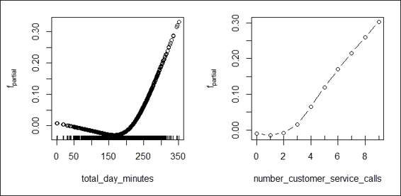
The partial contribution plot of important attributes

Calculating the margins of a classifier

A margin is a measure of the certainty of classification. This method calculates the difference between the support of a correct class and the maximum support of an incorrect class. In this recipe, we will demonstrate how to calculate the margins of the generated classifiers.

Getting ready

You need to have completed the previous recipe by storing a fitted bagging model in the variables, churn.bagging and churn.predbagging. Also, put the fitted boosting classifier in both churn.boost and churn.boost.pred.

How to do it...

Perform the following steps to calculate the margin of each ensemble learner:

1. First, use the margins function to calculate the margins of the boosting classifiers:

2. > boost.margins = margins(churn.boost, trainset)

3. > boost.pred.margins = margins(churn.boost.pred, testset)

2. You can then use the plot function to plot a marginal cumulative distribution graph of the boosting classifiers:

3. > plot(sort(boost.margins[[1]]), (1:length(boost.margins[[1]]))/length(boost.margins[[1]]), type="l",xlim=c(-1,1),main="Boosting: Margin cumulative distribution graph", xlab="margin", ylab="% observations", col = "blue")

4. > lines(sort(boost.pred.margins[[1]]), (1:length(boost.pred.margins[[1]]))/length(boost.pred.margins[[1]]), type="l", col = "green")

5. > abline(v=0, col="red",lty=2)

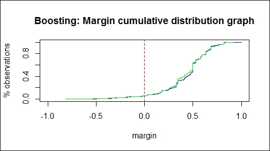
The margin cumulative distribution graph of using the boosting method

3. You can then calculate the percentage of negative margin matches training errors and the percentage of negative margin matches test errors:

4. > boosting.training.margin = table(boost.margins[[1]] > 0)

5. > boosting.negative.training = as.numeric(boosting.training.margin[1]/boosting.training.margin[2])

6. > boosting.negative.training

7. [1] 0.06387868

9. > boosting.testing.margin = table(boost.pred.margins[[1]] > 0)

10.> boosting.negative.testing = as.numeric(boosting.testing.margin[1]/boosting.testing.margin[2])

11.> boosting.negative.testing

12.[1] 0.06263048

4. Also, you can calculate the margins of the bagging classifiers. You might see the warning message showing "no non-missing argument to min". The message simply indicates that the min/max function is applied to the numeric of the 0 length argument:

5. > bagging.margins = margins(churn.bagging, trainset)

6. > bagging.pred.margins = margins(churn.predbagging, testset)

5. You can then use the plot function to plot a margin cumulative distribution graph of the bagging classifiers:

6. > plot(sort(bagging.margins[[1]]), (1:length(bagging.margins[[1]]))/length(bagging.margins[[1]]), type="l",xlim=c(-1,1),main="Bagging: Margin cumulative distribution graph", xlab="margin", ylab="% observations", col = "blue")

8. > lines(sort(bagging.pred.margins[[1]]), (1:length(bagging.pred.margins[[1]]))/length(bagging.pred.margins[[1]]), type="l", col = "green")

9. > abline(v=0, col="red",lty=2)

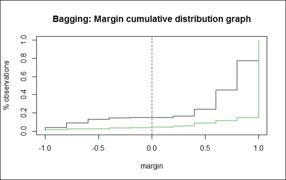
The margin cumulative distribution graph of the bagging method

6. Finally, you can then compute the percentage of negative margin matches training errors and the percentage of negative margin matches test errors:

7. > bagging.training.margin = table(bagging.margins[[1]] > 0)

8. > bagging.negative.training = as.numeric(bagging.training.margin[1]/bagging.training.margin[2])

9. > bagging.negative.training

10.[1] 0.1733401

11.

12.> bagging.testing.margin = table(bagging.pred.margins[[1]] > 0)

13.> bagging.negative.testing = as.numeric(bagging.testing.margin[1]/bagging.testing.margin[2])

14.> bagging.negative.testing

15.[1] 0.04303279

How it works...

A margin is the measurement of certainty of the classification; it is computed by the support of the correct class and the maximum support of the incorrect class. The formula of margins can be formulated as:

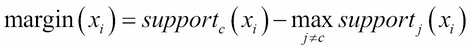
Here, the margin of the xi sample equals the support of a correctly classified sample (c denotes the correct class) minus the maximum support of a sample that is classified to class j (where j≠c and j=1…k). Therefore, correctly classified examples will have positive margins and misclassified examples will have negative margins. If the margin value is close to one, it means that correctly classified examples have a high degree of confidence. On the other hand, examples of uncertain classifications will have small margins.

The margins function calculates the margins of AdaBoost.M1, AdaBoost-SAMME, or the bagging classifier, which returns a vector of a margin. To visualize the margin distribution, one can use a margin cumulative distribution graph. In these graphs, the x-axis shows the margin and the y-axis shows the percentage of observations where the margin is less than or equal to the margin value of the x-axis. If every observation is correctly classified, the graph will show a vertical line at the margin equal to 1 (where margin = 1).

For the margin cumulative distribution graph of the boosting classifiers, we can see that there are two lines plotted on the graph, in which the green line denotes the margin of the testing dataset, and the blue line denotes the margin of the training set. The figure shows about 6.39 percent of negative margins match the training error, and 6.26 percent of negative margins match the test error. On the other hand, we can find that 17.33% of negative margins match the training error and 4.3 percent of negative margins match the test error in the margin cumulative distribution graph of the bagging classifiers. Normally, the percentage of negative margins matching the training error should be close to the percentage of negative margins that match the test error. As a result of this, we should then examine the reason why the percentage of negative margins that match the training error is much higher than the negative margins that match the test error.

See also

· If you are interested in more details on margin distribution graphs, please refer to the following source: Kuncheva LI (2004), Combining Pattern Classifiers: Methods and Algorithms, John Wiley & Sons.

Calculating the error evolution of the ensemble method

The adabag package provides the errorevol function for a user to estimate the ensemble method errors in accordance with the number of iterations. In this recipe, we will demonstrate how to use errorevol to show the evolution of errors of each ensemble classifier.

Getting ready

You need to have completed the previous recipe by storing the fitted bagging model in the variable, churn.bagging. Also, put the fitted boosting classifier in churn.boost.

How to do it...

Perform the following steps to calculate the error evolution of each ensemble learner:

1. First, use the errorevol function to calculate the error evolution of the boosting classifiers:

2. > boosting.evol.train = errorevol(churn.boost, trainset)

3. > boosting.evol.test = errorevol(churn.boost, testset)

4. > plot(boosting.evol.test$error, type = "l", ylim = c(0, 1),

5. + main = "Boosting error versus number of trees", xlab = "Iterations",

6. + ylab = "Error", col = "red", lwd = 2)

7. > lines(boosting.evol.train$error, cex = .5, col = "blue", lty = 2, lwd = 2)

8. > legend("topright", c("test", "train"), col = c("red", "blue"), lty = 1:2, lwd = 2)

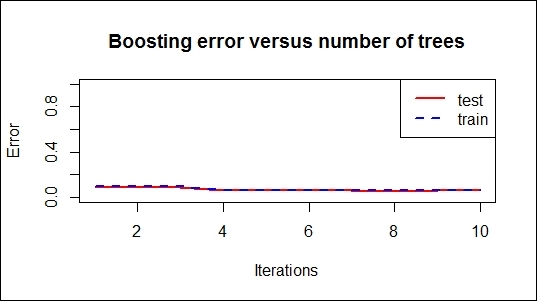
Boosting error versus number of trees

2. Next, use the errorevol function to calculate the error evolution of the bagging classifiers:

3. > bagging.evol.train = errorevol(churn.bagging, trainset)

4. > bagging.evol.test = errorevol(churn.bagging, testset)

5. > plot(bagging.evol.test$error, type = "l", ylim = c(0, 1),

6. + main = "Bagging error versus number of trees", xlab = "Iterations",

7. + ylab = "Error", col = "red", lwd = 2)

8. > lines(bagging.evol.train$error, cex = .5, col = "blue", lty = 2, lwd = 2)

9. > legend("topright", c("test", "train"), col = c("red", "blue"), lty = 1:2, lwd = 2)

Bagging error versus number of trees

How it works...

The errorest function calculates the error evolution of AdaBoost.M1, AdaBoost-SAMME, or the bagging classifiers and returns a vector of error evolutions. In this recipe, we use the boosting and bagging models to generate error evolution vectors and graph the error versus number of trees.

The resulting graph reveals the error rate of each iteration. The trend of the error rate can help measure how fast the errors reduce, while the number of iterations increases. In addition to this, the graphs may show whether the model is over-fitted.

See also

· If the ensemble model is over-fitted, you can use the predict.bagging and predict.boosting functions to prune the ensemble model. For more information, please use the help function to refer to predict.bagging and predict.boosting:

· > help(predict.bagging)

· > help(predict.boosting)

Classifying data with random forest

Random forest is another useful ensemble learning method that grows multiple decision trees during the training process. Each decision tree will output its own prediction results corresponding to the input. The forest will use the voting mechanism to select the most voted class as the prediction result. In this recipe, we will illustrate how to classify data using the randomForest package.

Getting ready

In this recipe, we will continue to use the telecom churn dataset as the input data source to perform classifications with the random forest method.

How to do it...

Perform the following steps to classify data with random forest:

1. First, you have to install and load the randomForest package;

2. > install.packages("randomForest")

3. > library(randomForest)

2. You can then fit the random forest classifier with a training set:

3. > churn.rf = randomForest(churn ~ ., data = trainset, importance = T)

4. > churn.rf

6. Call:

7. randomForest(formula = churn ~ ., data = trainset, importance = T)

8. Type of random forest: classification

9. Number of trees: 500

10.No. of variables tried at each split: 4

11.

12. OOB estimate of error rate: 4.88%

13.Confusion matrix:

14. yes no class.error

15.yes 247 95 0.277777778

16.no 18 1955 0.009123163

3. Next, make predictions based on the fitted model and testing dataset:

4. > churn.prediction = predict(churn.rf, testset)

4. Similar to other classification methods, you can obtain the classification table:

5. > table(churn.prediction, testset$churn)

7. churn.prediction yes no

8. yes 110 7

9. no 31 870

5. You can use the plot function to plot the mean square error of the forest object:

6. > plot(churn.rf)

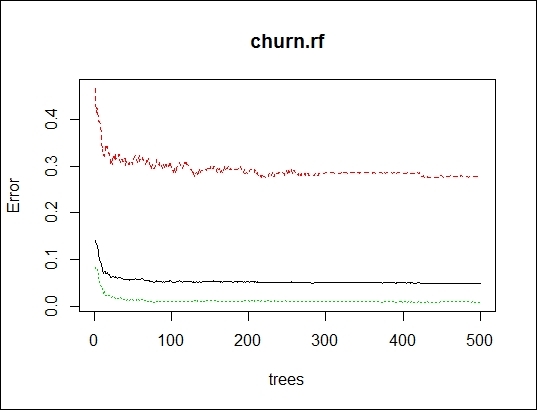
The mean square error of the random forest

6. You can then examine the importance of each attribute within the fitted classifier:

7. > importance(churn.rf)

8. yes no

9. international_plan 66.55206691 56.5100647

10.voice_mail_plan 19.98337191 15.2354970

11.number_vmail_messages 21.02976166 14.0707195

12.total_day_minutes 28.05190188 27.7570444

7. Next, you can use the varImpPlot function to obtain the plot of variable importance:

8. > varImpPlot(churn.rf)

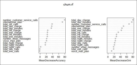
The visualization of variable importance

8. You can also use the margin function to calculate the margins and plot the margin cumulative distribution:

9. > margins.rf=margin(churn.rf,trainset)

10.> plot(margins.rf)

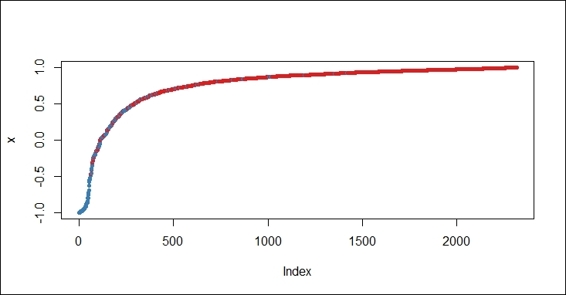
The margin cumulative distribution graph for the random forest method

9. Furthermore, you can use a histogram to visualize the margin distribution of the random forest:

10.> hist(margins.rf,main="Margins of Random Forest for churn dataset")

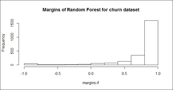
The histogram of margin distribution

10.You can also use boxplot to visualize the margins of the random forest by class:

11.> boxplot(margins.rf~trainset$churn, main="Margins of Random Forest for churn dataset by class")

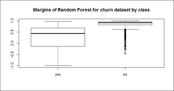
Margins of the random forest by class

How it works...

The purpose of random forest is to ensemble weak learners (for example, a single decision tree) into a strong learner. The process of developing a random forest is very similar to the bagging method, assuming that we have a training set containing N samples with M features. The process first performs bootstrap sampling, which samples N cases at random, with the replacement as the training dataset of each single decision tree. Next, in each node, the process first randomly selects m variables (where m << M), then finds the predictor variable that provides the best split among m variables. Next, the process grows the full tree without pruning. In the end, we can obtain the predicted result of an example from each single tree. As a result, we can get the prediction result by taking an average or weighted average (for regression) of an output or taking a majority vote (for classification):

A random forest uses two parameters: ntree (the number of trees) and mtry (the number of features used to find the best feature), while the bagging method only uses ntree as a parameter. Therefore, if we set mtry equal to the number of features within a training dataset, then the random forest is equal to the bagging method.

The main advantages of random forest are that it is easy to compute, it can efficiently process data, and is fault tolerant to missing or unbalanced data. The main disadvantage of random forest is that it cannot predict the value beyond the range of a training dataset. Also, it is prone to over-fitting of noisy data.

In this recipe, we employ the random forest method adapted from the randomForest package to fit a classification model. First, we install and load randomForest into an R session. We then use the random forest method to train a classification model. We set importance = T, which will ensure that the importance of the predictor is assessed.

Similar to the bagging and boosting methods, once the model is fitted, one can perform predictions using a fitted model on the testing dataset, and furthermore, obtain the classification table.

In order to assess the importance of each attribute, the randomForest package provides the importance and varImpPlot functions to either list the importance of each attribute in the fitted model or visualize the importance using either mean decrease accuracy or mean decrease gini.

Similar to adabag, which contains a method to calculate the margins of the bagging and boosting methods, randomForest provides the margin function to calculate the margins of the forest object. With the plot, hist, and boxplotfunctions, you can visualize the margins in different aspects to the proportion of correctly classified observations.

There's more...

Apart from the randomForest package, the party package also provides an implementation of random forest. In the following steps, we illustrate how to use the cforest function within the party package to perform classifications:

1. First, install and load the party package:

2. > install.packages("party")

3. > library(party)

2. You can then use the cforest function to fit the classification model:

3. > churn.cforest = cforest(churn ~ ., data = trainset, controls=cforest_unbiased(ntree=1000, mtry=5))

4. > churn.cforest

6. Random Forest using Conditional Inference Trees

8. Number of trees: 1000

10.Response: churn

11.Inputs: international_plan, voice_mail_plan, number_vmail_messages, total_day_minutes, total_day_calls, total_day_charge, total_eve_minutes, total_eve_calls, total_eve_charge, total_night_minutes, total_night_calls, total_night_charge, total_intl_minutes, total_intl_calls, total_intl_charge, number_customer_service_calls

12.Number of observations: 2315

3. You can make predictions based on the built model and the testing dataset:

4. > churn.cforest.prediction = predict(churn.cforest, testset, OOB=TRUE, type = "response")

4. Finally, obtain the classification table from the predicted labels and the labels of the testing dataset:

5. > table(churn.cforest.prediction, testset$churn)

7. churn.cforest.prediction yes no

8. yes 91 3

9. no 50 874

Estimating the prediction errors of different classifiers

At the beginning of this chapter, we discussed why we use ensemble learning and how it can improve the prediction performance compared to using just a single classifier. We now validate whether the ensemble model performs better than a single decision tree by comparing the performance of each method. In order to compare the different classifiers, we can perform a 10-fold cross-validation on each classification method to estimate test errors using erroreset from the ipred package.

Getting ready

In this recipe, we will continue to use the telecom churn dataset as the input data source to estimate the prediction errors of the different classifiers.

How to do it...

Perform the following steps to estimate the prediction errors of each classification method:

1. You can estimate the error rate of the bagging model:

2. > churn.bagging= errorest(churn ~ ., data = trainset, model = bagging)

3. > churn.bagging

5. Call:

6. errorest.data.frame(formula = churn ~ ., data = trainset, model = bagging)

8. 10-fold cross-validation estimator of misclassification error

10.Misclassification error: 0.0583

2. You can then estimate the error rate of the boosting method:

3. > install.packages("ada")

4. > library(ada)

5. > churn.boosting= errorest(churn ~ ., data = trainset, model = ada)

6. > churn.boosting

8. Call:

9. errorest.data.frame(formula = churn ~ ., data = trainset, model = ada)

10.

11. 10-fold cross-validation estimator of misclassification error

12.

13.Misclassification error: 0.0475

3. Next, estimate the error rate of the random forest model:

4. > churn.rf= errorest(churn ~ ., data = trainset, model = randomForest)

5. > churn.rf

7. Call:

8. errorest.data.frame(formula = churn ~ ., data = trainset, model = randomForest)

10. 10-fold cross-validation estimator of misclassification error

11.

12.Misclassification error: 0.051

4. Finally, make a prediction function using churn.predict, and then use the function to estimate the error rate of the single decision tree:

5. > churn.predict = function(object, newdata) {predict(object, newdata = newdata, type = "class")}

6. > churn.tree= errorest(churn ~ ., data = trainset, model = rpart,predict = churn.predict)

7. > churn.tree

9. Call:

10.errorest.data.frame(formula = churn ~ ., data = trainset, model = rpart,

11. predict = churn.predict)

12.

13. 10-fold cross-validation estimator of misclassification error

14.

15.Misclassification error: 0.0674

How it works...

In this recipe, we estimate the error rates of four different classifiers using the errorest function from the ipred package. We compare the boosting, bagging, and random forest methods, and the single decision tree classifier. The errorest function performs a 10-fold cross-validation on each classifier and calculates the misclassification error. The estimation results from the four chosen models reveal that the boosting method performs the best with the lowest error rate (0.0475). The random forest method has the second lowest error rate (0.051), while the bagging method has an error rate of 0.0583. The single decision tree classifier, rpart, performs the worst among the four methods with an error rate equal to 0.0674. These results show that all three ensemble learning methods, boosting, bagging, and random forest, outperform a single decision tree classifier.

See also

· In this recipe we mentioned the ada package, which contains a method to perform stochastic boosting. For those interested in this package, please refer to: Additive Logistic Regression: A Statistical View of Boosting by Friedman, et al. (2000).