R Recipes: A Problem-Solution Approach (2014)
Chapter 9. Probability Distributions
Looking up probabilities once was a time-consuming, complex, and error-prone task. Virtually every statistics book has tables of various probability distributions in an appendix, but R provides a family of functions for both discrete and continuous probability functions, making the use of tables unnecessary. You have already seen the rnorm() function used to produce random numbers that simulate a normal distribution with a certain mean and standard deviation. The functions for other probability distributions are all similarly labeled to make it easy to remember them.
In this chapter, you will learn how to use R for finding various probabilities for both discrete and continuous probability distributions. The normal distribution can serve as a model for the rest. The density function is dnorm(). The cumulative probability distribution (PDF) is pnorm()and the quantile function is qnorm(). The function for simulating a random value based on the normal distribution is rnorm().
Recipe 9-1. Finding Areas Under the Standard Normal Curve
Problem
Everyone who uses statistics on even a casual basis needs to look up the probability to the left or to the right of a given z score. It is also very common to need to find the area between two z scores. Because the standard normal distribution is symmetrical, many of the tables go from the mean of 0 to a high z score of 3.5 or 4.0. In Recipe 9-1, you learn how to build and plot your own standard normal distribution to visualize areas under the curve. You also learn how to “look up” areas and plot them for visualization.
Solution
First, we will build two vectors. One is the x axis (z scores ranging from –4 to 4) and the other is the probability density for each z score. This is the y axis. We will combine the vectors into a data frame, which we will abbreviate df. To get the densities, we use the dnorm() function.
> xaxis <- seq(-4, 4, by = 0.10)
> yaxis <- dnorm(xaxis)
> df <- as.data.frame(cbind(xaxis, yaxis))
We now have everything we need to build a standard normal distribution and plot it (see Figure 9-1). Here’s how to build the curve. Though technically not required, combining the axes into a data frame allows us to use ggplot2 with the data frame to produce different graphics. Here, however, we simply use the base R graphics module to plot the normal curve. To clarify matters, the type is "l", which stands for “line,” and not the numeral 1.
df <- as.data.frame(cbind(xaxis, yaxis))
> plot(df, xlab = "z score", ylab = "density", type = "l")
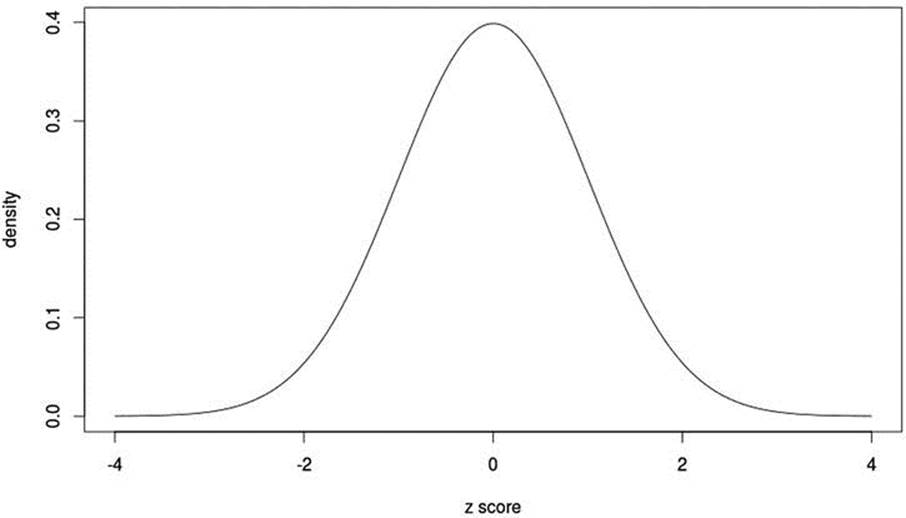
Figure 9-1. The standard normal curve
We see the familiar unimodal, symmetrical, bell-shaped curve and note that the probabilities taper off rapidly after values of z = ±3.
You can find areas under the normal curve by using a subtraction strategy. The pnorm() function also allows you to find both right- and left-tailed probabilities. You can find the area between any two z scores simply by subtracting the area to the left of the lower z score from the area to the left of the higher z score. Find the area to the left of a z score by using the pnorm() function. Similarly, you can find the area to the right of a given z score by setting the lower argument to FALSE (or by finding 1-pnorm()). Let us determine the areas to the left and right of a z score of 1.96:
> pnorm(1.96)
[1] 0.9750021
> pnorm(1.96, lower = FALSE)
[1] 0.0249979
Clearly, if we subtract the area to the left of z = –1.96 from the area to the left of z =1.96, we will be left with the middle 95% of the standard normal distribution:
> pnorm(1.96) - pnorm(1.96, lower = FALSE)
[1] 0.9500042
We could also find this using pnorm(1.96)-pnorm(-1.96).
It is similarly easy to use the qnorm() function to locate critical values. Assume we want the value of z that cuts off the top 10% of the standard normal distribution from the lower 90%. We use the qnorm() function as follows:
> qnorm(.90)
[1] 1.281552
We can also supply a vector of quantiles to the qnorm() function. For example, here are the critical values of z for alpha levels of .10, .05, and .01.
> quantiles <- c(.95, .975, .995)
> qnorm(quantiles)
[1] 1.644854 1.959964 2.575829
Recipe 9-2. Working with Binomial Probabilities
The binomial probability distribution is the distribution of the random variable r, the number of “successes” in a series of N dichotomous (0,1) trials, where the result of each trial is a 0 (failure) or a 1 (success). Often the definition of success is arbitrary, as in heads or tails in a coin toss, but sometimes the definition of success is logical, as in a correct answer to a multiple-choice question or a unit without a defect. The binomial distribution gives the probability of r successes in N trials, where r can range from 0 to N. The most common and well-known example is that of a coin toss. We know intuitively that a fair coin has a probability of .5 of landing on heads, and a probability of .5 of landing on tails. Yet when we flip the coin, we get one or the other. The two outcomes are dbinom mutually exclusive. The law of large numbers tells us that over a long series of trials, the empirical probability of heads will converge on the theoretical probability.
Problem
Technically, the binomial probability distribution has a probability mass function (PMF), rather than a PDF, because the binomial distribution is discrete. Finding binomial probabilities is similar to finding normal probabilities.
Solution
The binomial distribution is used in a variety of applications. Binomial distributions have the following four characteristics:
· The probability of success, p, remains constant for all trials.
· The procedure has a fixed number of trials, N.
· The N trials are independent. The outcome of any trial does not affect the outcome of any other trial.
· Each trial must result in either a success or a failure.
As an example, assume that a manufacturing process is known to produce 4.7% defective parts. A random sample of 10 parts is obtained. What is the probability that exactly 3 parts are defective? What is the probability that 0 parts are defective? What is the probability that 4 or more parts are defective? The binomial distribution can help us answer these questions. For the sake of illustration, let us generate the entire distribution of binomial probabilities for exactly 0 to 10 defective parts given a defect rate of .047. We use the dbinom() function in this case. For convenience, we create a data frame to show the number of “successes” (in this case, defects) and the exact probabilities.
> r <- 0:10
> N <- 10
> p <- .047
> prob <- round(dbinom(r, N, p), 5)
> prob <- as.data.frame(cbind(r, prob))
> prob
r prob
1 0 0.61792
2 1 0.30474
3 2 0.06763
4 3 0.00889
5 4 0.00077
6 5 0.00005
7 6 0.00000
8 7 0.00000
9 8 0.00000
10 9 0.00000
11 10 0.00000
The probability of exactly 3 parts being defective is .06763. The probability of exactly 0 parts being defective is .61792. The probability of 4 or more parts being defective is .00077 + .00005 = .00083. We can also use the cumulative binomial distribution to solve the last problem, the probability of 4 or more parts being defective. The complement rule of probability says that we can find the complement of a probability p by subtracting p from 1. We can find the left-tailed probability of r | R <= 3 as follows, and then subtract that value from 1 to get the probability of 4 or more defects.
> round(1 - pbinom(3, 10, .047), 5)
[1] 0.00082
As another example, assume that a commercial airliner has four jet engines. The independent reliability of each engine is p = .92 or 92%. For the aircraft to land safely, at least two of the engines must be working properly. What is the probability that the flight can land safely? The probability that two or more engines will work properly is .998 or 99.8%. We can find this using the complement rule, or equivalently by setting the lower argument to F or FALSE:
> N <- 4
> p <- .92
> 1 - pbinom(1, N, p)
[1] 0.9980749
> pbinom(1, N, p, lower = F)
[1] 0.9980749
Recipe 9-3. Working with Poisson Probabilities
Problem
The Poisson distribution (named after French mathematician Siméon Denis Poisson) shows the number of “occurrences” within a given interval. The interval may be distance, time, area, volume, or some other measure. Unlike the binomial distribution, the Poisson distribution does not have a fixed number of observations. The Poisson distribution applies in the following circumstances:
· The number of occurrences that occur within a given interval is independent of the number of occurrences in any other nonoverlapping interval.
· The probability that an occurrence will fall within an interval is the same for all intervals of the same size, and is proportional to the size of the interval (for small intervals).
· As the size of the interval becomes smaller, the probability of an occurrence in that interval approaches zero.
Remember the Poisson counts have no theoretical upper bound, so we often use the complement rule of probability to solve Poisson problems. In many disciplines, certain events need to be counted or estimated in order to make good decisions or plans. For example, the number of cars going through an intersection, or the number of accidents at the intersection could be a justification for installing a traffic light. Estimating the number of calls arriving at a customer service center is important for staffing purposes.
Solution
The Poisson distribution is useful for determining probabilities of events that occur rarely, but are significant when they do occur. One of the earliest applications of the Poisson distribution was its use by Ladislaus Bortkiewicz in 1898 to study the rate of deaths among Prussian soldiers who had been accidentally kicked by horses.
In more routine applications, the Poisson distribution has been used to determine the probabilities of industrial accidents, hurricanes, and manufacturing defects. As an example, imagine that a manufacturing plant has historically averaged six “reportable” accidents per quarter. What is the probability of exactly six accidents in the next quarter? What is the probability of zero accidents? What is the probability of more than six accidents? We can use the functions for the Poisson distribution to answer these questions. We must supply the number of occurrences (which can be a vector) and lambda (which is the mean number of occurrences per interval). Following the pattern of binomial probabilities, dpois(x,lambda) gives the probability that there are x occurrences in an interval, while ppois(x,lambda) gives the probability of x or fewer occurrences in an interval, when the mean occurrence rate for intervals of that size is lambda.
> dpois(6, 6) ## The exact probability of 6 accidents
[1] 0.1606231
> dpois(0, 6) ## The exact probability of 0 accidents
[1] 0.002478752
> 1 - ppois (6, 6) ## The probability of more than 6 accidents
[1] 0.3936972
Recipe 9-4. Finding p Values and Critical Values of t, F, and Chi-Square
Problem
P values and critical values figure prominently in inferential statistics. Historically, tables of critical values were used to determine the significance of a statistical test and to choose the appropriate values for developing confidence intervals. Tables are helpful, but often incomplete, and the use of tables is often cumbersome and prone to error. You saw earlier that the qnorm() function can be used to find critical values of z for different alpha levels. We can similarly use qt(), qf(), and qchisq() for finding critical values of t, F, and chi-square for various degrees of freedom. The built-in functions of R make tables largely unnecessary, as these functions are faster to use and often more accurate than tabled values.
Solution
Finding quantiles for various probability distributions is very easy. You may recall the t distribution has a single parameter: the degrees of freedom. The F distribution has two parameters: the degrees of freedom for the numerator and the degrees of freedom for the denominator. The chi-square distribution has one parameter: the degrees of freedom. Interestingly from a mathematical standpoint, each of these distributions has a theoretical relationship to the normal distribution, though their probability density functions are quite different from that for the normal distribution. The t distribution is symmetrical, like the normal distribution, but the F and chi-square distributions are positively skewed.
Finding p Values for t
Finding one- and two-tailed p values for t is made simple with the pt() function. The pt() function returns the left-tailed, or optionally, the right-tailed cumulative probability for a given value of t and the relevant degrees of freedom. For example, if we have conducted a one-tailed test with 18 degrees of freedom, and the value of t calculated from our sample results was 2.393, the p value is found as follows:
> pt(2.393, 18, lower = F)
[1] 0.01391179
If the test is two-tailed, we can simply double the one-tailed probability:
> 2 * pt(2.393, 18, lower = F)
[1] 0.02782358
Finding Critical Values of t
For t tests, we often use two-tailed hypothesis tests, and for such tests, there will be two critical values of t. We also use lower and upper critical values of t to develop confidence intervals for the mean. It is typical practice to use only the right tail of the F and chi-square distributions for hypothesis tests, but in certain circumstances, we use both tails, as in confidence intervals for the variance and standard deviation using the chi-square distribution.
Assume we have the following 25 scores:
> x <- rnorm(25, 65, 10)
> x <- round(x, 1)
> x
[1] 60.2 64.4 64.8 65.6 63.7 68.0 85.7 58.2 53.1 55.0 72.3 50.2 78.5 67.1 79.2
[16] 72.1 59.2 50.6 77.8 56.3 64.0 76.8 68.2 75.0 59.6
We can use the t distribution to develop a confidence interval for the population mean. Because we have 25 scores, the degrees of freedom are n – 1 = 24. We want to find the values of t that cut off the top 2.5% of the distribution and the lower 2.5%, leaving us with 95% in the middle. Like the standard normal distribution, the t distribution has a mean of zero. Because the t distribution is an estimate of the normal distribution, a confidence interval based on the t distribution will be wider than a confidence interval based on the standard normal distribution. Let us calculate the mean and standard deviation of the data, and then construct a confidence interval. We will use the fBasics package. Begin with the commands install.packages("fBasics") and library(fBasics).
> install.packages("fBasics")
> library(fBasics)
> basicStats(x)
x
nobs 25.000000
NAs 0.000000
Minimum 50.200000
Maximum 85.700000
1. Quartile 59.200000
3. Quartile 72.300000
Mean 65.824000
Median 64.800000
Sum 1645.600000
SE Mean 1.917057
LCL Mean 61.867388
UCL Mean 69.780612
Variance 91.877733
Stdev 9.585287
Skewness 0.178608
Kurtosis -0.968359
Note the upper (UCL) and lower (LCL) control limits of the 95% confidence interval for the mean. These are developed using the t distribution. The confidence interval can be defined as:
95% CI: M – tα/2×sM ≤ μ ≤ M + tα/2×sM
We can use the qt() function to find the critical values of t as follows. As with the normal distribution, the critical values of t are the same in absolute value. The value sM is the standard error of the mean, which is reported above.
> qt(.975, 24)
[1] 2.063899
> qt(.025, 24)
[1] -2.063899
Substituting the appropriate values produces the following result, and we see that our confidence limits agree with those produced by the fBasics package.
95% CI = 65.824 – 2.063899×1.917057 ≤ μ ≤ 65.824 + 2.063899×1.917057
= 65.824 – 3.956612 ≤ μ ≤ 65.824 + 3.956612
= 61.867388 ≤ μ ≤ 69.780612
The t.test() function in R will automatically produce confidence intervals. For example, if we simply do a one-sample t test with the preceding data, R will calculate the confidence interval for us:
> t.test(x)
One Sample t-test
data: x
t = 34.336, df = 24, p-value < 2.2e-16
alternative hypothesis: true mean is not equal to 0
95 percent confidence interval:
61.86739 69.78061
sample estimates:
mean of x
65.824
Finding p Values for F
Unlike the t distribution, the F distribution is positively skewed. It has two degrees of freedom so most textbooks have several pages of tables, which could be eliminated using R. As I mentioned earlier, we usually find critical values of F in the right tail of the distribution. The F ratio is formed from two variance estimates, and it can range from zero to +∞. As a matter of expediency, if you are simply testing the equality of two variance estimates, you should always divide the smaller estimate into the larger one. Though it is possible to test using the left tail of the Fdistribution, this is rarely done. The pf() function locates the p value and the qf() function gives the quantile for a given F ratio and the relevant degrees of freedom.
For example, assume we have two variance estimates and wish to test the null hypothesis that they are equal against the alternative that they are unequal. Let’s create a vector of y scores to join with the x scores we worked with in Recipe 9-4:
> head(df)
x y
1 60.2 84.5
2 64.4 89.7
3 64.8 74.0
4 65.6 90.4
5 63.7 84.9
6 68.0 99.6
> tail(df)
x y
20 56.3 79.8
21 64.0 82.5
22 76.8 80.7
23 68.2 86.4
24 75.0 81.2
25 59.6 94.1
We can use the sapply() function to obtain the variances of x and y.
> sapply(df, var)
x y
91.87773 43.40677
The question is whether the variance for x, the larger of the two estimates, is significantly larger than the variance for y. There are 25 observations for each variable, so the degrees of freedom for the F ratio are 24 and 24. We supply the value of F, the numerator degrees of freedom, and the denominator degrees of freedom to find the p value. To obtain a two-tailed p value, we double the one-tailed value:
F <- var(x)/var(y)
> F
[1] 2.075825
> pvalue
Error: object 'pvalue' not found
> pvalue <- 2*(pf(F, 24, 24, lower = FALSE)
+ )
> pvalue
[1] 0.07984798
We see that the estimates differ by more than a factor of 2, but they are not significantly different at alpha = .05. To compare the means of x and y, we could therefore use the t test that assumes equality of variance. The two means are significantly different, as the p value indicates.
> t.test(x, y, var.equal = T)
Two Sample t-test
data: x and y
t = -8.7317, df = 48, p-value = 1.766e-11
alternative hypothesis: true difference in means is not equal to 0
95 percent confidence interval:
-25.06795 -15.68405
sample estimates:
mean of x mean of y
65.824 86.200
Finding Critical Values of F
Use the qf() function to find quantiles for the F distribution. For example, assume we have three groups and each group has 10 observations. For an analysis of variance, the critical value of F would be found as follows. Note we have 29 total degrees of freedom, 2 degrees of freedom between groups, and 27 degrees of freedom within groups. We thus need a critical value of F for 2 and 27 degrees of freedom that cut off the lower 95% of the F distribution from the upper 5%:
> qf(0.95, 2, 27)
[1] 3.354131
Finding p Values for Chi-Square
The chi-square distribution, like the F distribution, is positively skewed. It has one parameter, the degrees of freedom. We use the chi-square distribution nonparametrically for tests of model fit (or goodness of fit) and association. The chi-square distribution is also used parametrically for confidence intervals for the variance and standard deviation.
Use the pchisq() function to find the p value for a value of chi-square. In an interesting historical side note, Pearson, who developed the chi-square tests of goodness of fit and association, had difficulty with getting the degrees of freedom right. Fisher corrected Pearson—and the two were bitter enemies thereafter. For chi-square used for goodness of fit, the degrees of freedom are not based on sample size, but on the number of categories. We will discuss this in more depth in Chapter 10.
Assume we have a value of chi-square of 16.402 with 2 degrees of freedom. Find the p value as follows:
> chisq <- 16.402
> pchisq(chisq, 2, lower = FALSE)
[1] 0.0002743791
Finding Critical Values of Chi-Square
We can use the qchisq() function for finding critical values of chi-square. For tests of goodness of fit and association (also known as tests of independence), we test on the right tail of the distribution. For confidence intervals for the variance and the standard deviation, we find left- and right-tailed values of chi-square.
Now, let us see how to construct a confidence interval for the population variance using the chi-square distribution. We will use the standard 95% confidence interval. We will continue to work with our example data. We found the variance for x from our previous table to be 91.87773. A confidence interval for the population variance can be defined as follows:
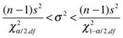
The right and left values of chi-square cut off the upper and lower 2.5% of the distribution, respectively. Let us find both values. We supply the probability and the degrees of freedom. In this case, the degrees of freedom are n – 1 = 25 – 1 = 24.
> qchisq(.975, 24)
[1] 39.36408
> qchisq(.025, 24)
[1] 12.40115
Now, we can substitute the required values to find the confidence interval for the population variance:
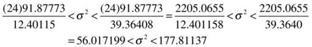
To find the confidence interval for the standard deviation, simply extract the positive square roots of the upper and lower limits:
![]()