R Recipes: A Problem-Solution Approach (2014)

Chapter 10. Hypothesis Tests for Means, Ranks, or Proportions

R provides easy access to virtually any of the traditional hypothesis tests for means, ranks, and proportions one might need. In Chapter 10 you learn how to do hypothesis tests for one sample, for two samples, and for three or more samples. We will include both parametric tests and nonparametric tests, illustrating each with appropriate data. The statistics functions in base R are usually adequate, but it is often helpful to use additional packages for their enhanced features.

Before we delve into hypothesis testing, let us briefly review the scales of measurement and their relationship to data and hypothesis testing. Throughout this book, we have made little distinction between interval and ratio data. The difference, of course, is that ratio data have a true zero point, while the zero point on an interval scale is arbitrary. From a statistical perspective, we combine interval and ratio data into a single category, and we can do parametric statistical analyses with such data as long as the distributional assumptions are warranted. We have also used nominal data, which in the strictest sense are simply categories in which we group objects or individuals with the same attribute. We can use numbers to represent the categories, but a label or some other identifier would work as well. We have a variety of techniques for dealing with nominal data. Between nominal and interval data is the ordinal scale. Ordinal measures give us information about ranks, but they do not tell us about the differences between ranks. Because there are no equal intervals with ordinal data, we must use techniques based on the order of the measures. These techniques are generally called nonparametric because they require few, if any, assumptions about population parameters. Moreover, these techniques are not typically used to make estimates or inferences about population parameters.

Recipe 10-1. One-Sample Tests

Problem

Many studies are descriptive in nature and involve the collection of a single sample of data. Often there are no inferences involved in such studies. With descriptive studies, we summarize the data, perhaps graphically as well as numerically, and report our findings. In other studies, however, we are interested in comparing sample values to known or hypothesized population values. In such cases, we use a category of tests known as one-sample tests.

Solution

We will discuss one-sample tests for interval and ratio data, and then expand our discussion to include one-sample tests for ordinal and nominal data.

One-Sample z and t Tests for Means

When we describe a sample, we are typically interested in the standard descriptive statistics, including central tendency and variability. You learned to calculate these statistics in Chapter 7. As a quick reminder, we must have interval or ratio data for statistics such as the mean and variance to be meaningful. When we have such data, we can use the fBasics package to get a quick statistical summary. Here again are the summary statistics for the variable x we used in Chapter 9.

> require(fBasics)
Loading required package: fBasics
Loading required package: MASS
Loading required package: timeDate
Loading required package: timeSeries
> x
[1] 60.2 64.4 64.8 65.6 63.7 68.0 85.7 58.2 53.1 55.0 72.3 50.2 78.5 67.1 79.2
[16] 72.1 59.2 50.6 77.8 56.3 64.0 76.8 68.2 75.0 59.6
> basicStats(x)
x
nobs 25.000000
NAs 0.000000
Minimum 50.200000
Maximum 85.700000
1. Quartile 59.200000
3. Quartile 72.300000
Mean 65.824000
Median 64.800000
Sum 1645.600000
SE Mean 1.917057
LCL Mean 61.867388
UCL Mean 69.780612
Variance 91.877733
Stdev 9.585287
Skewness 0.178608
Kurtosis -0.968359

In situations where we know the population standard deviation, σ, we can use a z test to compare a sample mean to a known or hypothesized population mean. The one-sample z test is among the simplest of the hypothesis tests, and is typically the first parametric test taught in a statistics course. Assume that we know the population from which the x scores were sampled is normally distributed and has a standard deviation of 11. We want to test the hypothesis that the sample came from a population with a mean of 70. The one-sample z test is not built into the base version of R, but its calculations are relatively simple. We use the following formula, in which the known or hypothesized population mean is subtracted from the sample mean, and the difference is divided by the standard error of the mean.

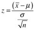
Assuming we want to do a two-tailed test with alpha = .05, we will use critical values of z = ±1.96. Our simple calculations are as follows:

> z <- (mean(x)- 70)/(11/sqrt(25))
> z
[1] -1.898182

If you want to create a more effective and reusable z.test function, you can do something like the following. The arguments supplied to the function are the raw data, the test value (mu), the sample size, and the alpha level, which is defaulted to the customary α = .05.

}

z.test <- function(x, mu, sigma, n, alpha = 0.05) {
sampleMean <- mean(x)
stdError <- sigma/sqrt(n)
zCrit <- qnorm(1 - alpha/2)
sampleZ <- (sampleMean-mu)/stdError
LL <- sampleMean - zCrit*stdError
UL <- sampleMean + zCrit*stdError
pValue <- 2 * (1 - pnorm(abs(sampleZ)))
cat("\t","one-sample z test","\n")
cat("sample mean:",sampleMean,"\n")
cat("test value:",mu,"\t","sigma:",sigma,"\n")
cat("sample z:",sampleZ,"\n")
cat("p value:",pValue,"\n")
cat((1-alpha)*100,"percent confidence interval","\n")
cat("lower:",LL,"\t","upper:",UL,"\n")
}

Here is the output from the z.test function shown earlier. For familiarity’s sake, I purposely produced output similar to that of the built-in t.test function in R.

> z.test(x, mu = 70, sigma = 11, n = 25, alpha = 0.05)
one-sample z test
sample mean: 65.824
test value: 70 sigma: 11
sample z: -1.898182
p value: 0.05767214
95 percent confidence interval
lower: 61.51208 upper: 70.13592

Because you now have a reusable function, you can change the arguments and run the test again. For example, let us change the alpha level to .01 and examine the new confidence interval. Note that as the confidence level increases, the interval width increases correspondingly.

> z.test(x,70,11,25,.01)
One-Sample z Test

sample mean: 65.824
test value: 70 sigma: 11
Sample z: -1.898182
P value: 0.05767214
99 percent confidence interval
Lower: 60.15718 Upper: 71.49082

The one-sample and two-sample z tests for means are implemented in the BSDA package available through CRAN. We will illustrate the BSDA package in Recipe 10-3.

It is rarely the case that we know the population standard deviation. When the population standard deviation is unknown, we use one-sample t tests to test hypotheses about a sample mean. The formula for t is identical to that for z, but we use the t distribution rather than the standard normal distribution to find p values and calculate confidence intervals, and we use the sample standard deviation instead of the population standard deviation. The t.test function allows you to test a sample mean against a known or hypothesized population mean when the population standard deviation is unknown. The function performs the t test and calculates a 95% confidence interval. The user specifies the data and the hypothesized population mean.

> t.test(x, mu = 70)

One Sample t-test

data: x
t = -2.1783, df = 24, p-value = 0.03943
alternative hypothesis: true mean is not equal to 70
95 percent confidence interval:
61.86739 69.78061
sample estimates:
mean of x
65.824

One-Sample Tests for Nominal and Ordinal Data

It is often of interest to determine whether a sample proportion is equal to a known or hypothesized population proportion. For example, a recent Gallup poll showed that 58% of Americans believe higher insurance rates are justified for those who smoke. Assume we conduct the same poll with a random sample in a tobacco-producing state such as North Carolina. We poll 300 adults and determine that 148 of them are in favor of higher insurance rates for smokers. Our sample proportion is as follows:

We can use the prop.test function in base R to determine whether the sample proportion of .4933 is significantly different from the hypothesized population proportion of .58:

> prop.test(148, 300, .58)

1-sample proportions test with continuity correction

data: 148 out of 300, null probability 0.58
X-squared = 8.8978, df = 1, p-value = 0.002855
alternative hypothesis: true p is not equal to 0.58
95 percent confidence interval:
0.4355593 0.5512809
sample estimates:
p
0.4933333

The results indicate that the sample proportion is significantly lower than the US average.

As a statistical side note, most statistics texts cast the one-sample test of proportion as a z test rather than a chi-square test. The interested reader is referred to a good statistics text for an explanation. A good online source for basic statistics is Dr. David Lane’s HyperStat web site athttp://davidmlane.com/hyperstat/.

‘Suffice it to say here that when one calculates z for a one-sample test of proportion, squaring the value of z produces the value of chi-square, and the two tests are statistically and mathematically equivalent. The binom.test function can be used for a proportion, as follows. Note, however, that the prop.test function applies the Yates correction for continuity, so the value of z² will not equal chi-square in this case, and the p values and confidence intervals are slightly different for the two tests, though not appreciably so:

> binom.test(148, 300, .58)

Exact binomial test

data: 148 and 300
number of successes = 148, number of trials = 300, p-value = 0.002797
alternative hypothesis: true probability of success is not equal to 0.58
95 percent confidence interval:
0.4354025 0.5513971
sample estimates:
probability of success
0.4933333

The paired-samples t test can be used to compare two scores for either the same subjects (repeated measures) or matched pairs of scores. The paired-samples t test is a special case of the one-sample t test in that the data of interest are the differences between the paired scores. Similarly, when you have ordinal data, a nonparametric alternative to the one-sample t test is the Wilcoxon signed rank test, which also applies to paired data. The paired-samples t test typically is used to test the hypothesis that the mean difference is zero against the alternative that the mean difference is not zero. Scale data that have been converted to ranks because the data are non-normal or data collected as ranks originally may be analyzed with the Wilcoxon signed rank test.

Assume there is a proposal to build a new school in a residential neighborhood. At the last town council meeting, results of a poll of 13 people in the neighborhood were presented as evidence that there is support for the new school. Unfortunately, the data collection tool was developed by one of the neighborhood residents, and yielded only ordinal data. Here are 13 hypothetical responses (see Table 10-1). Nine of the 13 respondents indicated the school should be built either immediately or soon. There is ordinality to the responses, but they are not on an interval scale. We can transform the responses to ordinal scores from 1 to 5 and test the hypothesis that the average score is 3 (no opinion) against the alternative that the median score is not equal to 3 (no opinion). We see that resident 8 has no opinion. The customary practice is to discard observations that lead to a zero difference between the score and the test value, so we will create the data frame omitting resident 8.

Table 10-1. Hypothetical Opinion Poll Results

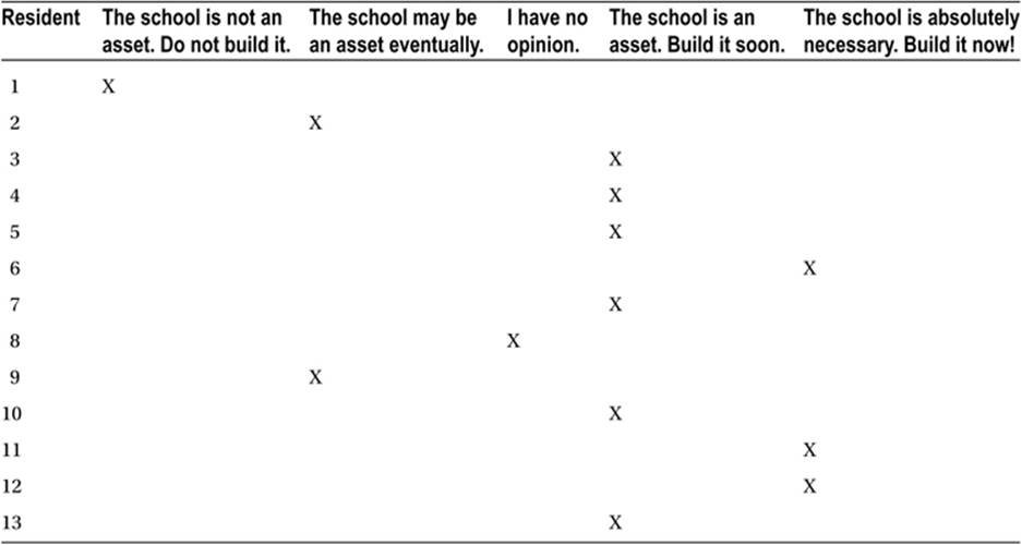
The transformed scores are as follows. I included a column for the test value, 3, and the difference between the individual’s ranking and the test value for instructive purposes, but these are not used in the test. Instead, one specifies the column of scores and the test value in the arguments to the wilcox.test function. Although the test value is technically a hypothetical median score, the function labels this as mu.

> schoolPoll
person score testValue diff
1 1 1 3 -2
2 2 2 3 -1
3 3 4 3 1
4 4 4 3 1
5 5 4 3 1
6 6 5 3 2
7 7 4 3 1
9 9 2 3 -1
10 10 4 3 1
11 11 5 3 2
12 12 5 3 2
13 13 4 3 1

> wilcox.test(schoolPoll$score, mu = 3)

Wilcoxon signed rank test with continuity correction

data: schoolPoll$score
V = 58.5, p-value = 0.1217
alternative hypothesis: true location is not equal to 3

Warning message:
In wilcox.test.default(schoolPoll$score, mu = 3) :
cannot compute exact p-value with ties

The test shows that the median score is not significantly different from the test value of 3. For the sake of comparison, the output from SPSS for the Wilcoxon signed rank test for the same data is shown in Figure 10-1. Unsurprisingly, the two programs produce the same result. The inquisitive reader may want to repeat this test using the column of difference scores as the data and with the test value set to zero. The results should be identical to those of the test on the scores themselves.

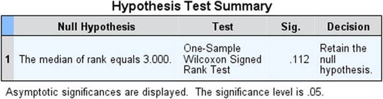
Figure 10-1. SPSS output for the Wilcoxon signed rank test

Recipe 10-2. Two-Sample Tests for Related Means, Ranks, and Proportions

Problem

Two-sample tests are many researchers’ stock in trade. The independent-samples t test is probably the most frequently used hypothesis test in many fields of research. We have discussed the one-sample t test and its relationship to the paired-samples t test, but let’s illustrate it again here. We will also discuss the independent-samples t tests, both assuming equal variances in the population and assuming unequal variances. Finally, we will discuss nonparametric tests for two samples using nominal and ordinal data.

Solution

The paired-samples t test is a special case of the one-sample t test, as we have discussed. Just as we did with the imaginary poll data in Recipe 10-1, we can calculate a column of difference scores for the pairs of observations. Testing the hypothesis that the mean difference is zero shows that there is really just one sample, the difference scores. The degrees of freedom correspond to the number of pairs minus 1, rather than the total number of observations.

With ordinal data, the Wilcoxon signed rank test illustrated in Recipe 10-1 can be used for paired data as well. The McNemar test is used for paired nominal data. As with the 2 × 2 chi-square test for independent samples, the McNemar test is often used in conjunction with the Yates continuity correction.

Let us begin with an example of a paired-samples t test. In this experiment conducted by the author, five-letter stimulus words were flashed briefly on a computer screen to the right or the left of a fixation point in the center of the screen. The duration of the word on the screen increased until the participant could type the correct word. Because of the “wiring” of the human brain, words projected to the left of the fixation point are sent to the right cerebral cortex for processing, whereas those shown on the right of the fixation point go to the left side. On the premise that the left side of the brain is specialized for verbal processing, it should be true that words are recognized more quickly by the left brain than by the right brain. Words sent to the right brain should take longer to be processed because of the extra time required to transfer them to the verbal processing areas on the left side of the brain. The data are as follows:

> head(pairedData)
sex age handed left right
1 M 24 R 0.115 0.139
2 F 19 R 0.090 0.093
3 F 22 L 0.104 0.133
4 F 18 L 0.101 0.100
5 F 18 L 0.116 0.116
6 F 18 L 0.090 0.113
> tail(pairedData)
sex age handed left right
92 F 18 R 0.093 0.096
93 F 19 R 0.106 0.124
94 F 20 R 0.093 0.099
95 F 18 R 0.108 0.108
96 M 18 R 0.110 0.136
97 M 18 R 0.098 0.116

For instructive purposes, let us once again calculate a column of difference scores, subtracting the processing time for the left side of the brain from that of the right side of the brain. We will append this column to the data frame by use of the cbind() function. As we suspected, most of the differences are positive, indicating the left side of the brain recognizes words more quickly than the right side does.

> diff <- pairedData$right - pairedData$left
> pairedData <- cbind(pairedData, diff)
> head(pairedData)
sex age handed left right diff
1 M 24 R 0.115 0.139 0.024
2 F 19 R 0.090 0.093 0.003
3 F 22 L 0.104 0.133 0.029
4 F 18 L 0.101 0.100 -0.001
5 F 18 L 0.116 0.116 0.000
6 F 18 L 0.090 0.113 0.023

Now, let us perform a paired-samples t test followed by a one-sample t test on the difference scores testing the hypothesis that the mean difference is zero against the two-sided alternative that the mean difference is not zero. Note that apart from slight labelling differences, the two tests produce the same results. The left side of the brain is significantly faster than the right side at recognizing words.

> t.test(pairedData$right, pairedData$left, paired = T)

Paired t-test

data: pairedData$right and pairedData$left
t = 7.6137, df = 96, p-value = 1.85e-11
alternative hypothesis: true difference in means is not equal to 0
95 percent confidence interval:
0.007362381 0.012555144
sample estimates:
mean of the differences
0.009958763

> t.test(pairedData$diff, mu = 0)

One Sample t-test

data: pairedData$diff
t = 7.6137, df = 96, p-value = 1.85e-11
alternative hypothesis: true mean is not equal to 0
95 percent confidence interval:
0.007362381 0.012555144
sample estimates:
mean of x
0.009958763

The data for both left- and right-brain word recognition are positively skewed. The difference data, however, are more normally distributed, as the histograms and normal q-q plot indicate (see Figure 10-2). Remember you can set the graphic device to show multiple graphs using the parfunction. We display histograms for the left- and right-brain word recognition data and the difference data, as well as a normal q-q plot for the difference data.

> par(mfrow=c(2,2))
> hist(pairedData$left)
> hist(pairedData$right)
> hist(pairedData$diff)
> qqnorm(pairedData$diff)

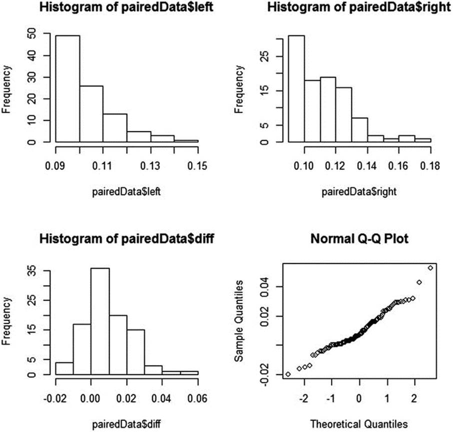
Figure 10-2. Histograms of the word recognition data

We can use the same data to illustrate the Wilcoxon signed rank test for paired data. The normal q-q plot shown in Figure 10-2 indicates a roughly linear relationship between the observed and theoretical quantiles, but the histogram shows the difference data are still slightly positively skewed and that there are outliers in the data. We can convert the data to ranks and then perform the signed rank test to determine if the average difference has a “location shift” of zero. This is the rough equivalent of testing the hypothesis that the median difference score is zero. Our paired-samples t test has already indicated that the left side of the brain is significantly faster at word recognition than the right side. Let us determine whether the difference is still significant when we use the nonparametric test. The signed rank test is significant.

> wilcox.test(pairedData$right, pairedData$left, paired = T)

Wilcoxon signed rank test with continuity correction

data: pairedData$right and pairedData$left
V = 3718, p-value = 1.265e-10
alternative hypothesis: true location shift is not equal to 0

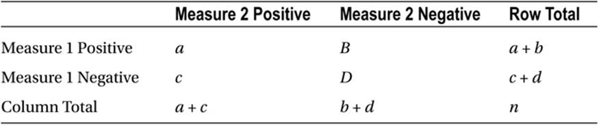
For nominal data, we can use the McNemar test for nominal data representing repeated measurements of the same objects or individuals or matched pairs of subjects. This test applies to 2 × 2 contingency tables in which the data are paired. The table is constructed as follows (see Table 10-2).

Table 10-2. Table Layout for the McNemar Test

The test statistic is chi-square with 1 degree of freedom, calculated as follows:

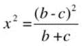
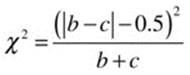
Note that the main diagonal of the table is not used to calculate the value of chi-square. Instead, the off-diagonal entries are used. We are testing the hypothesis that the off-diagonal entries b and c are equal. As with the 2 × 2 contingency table for independent samples, the Yates continuity correction may be applied, in which case the value of chi-square is computed as follows:

As a concrete example, assume we asked a sample of 1,009 people whether they approved or disapproved of George W. Bush’s handling of his job as president immediately before and immediately after the September 11 attacks. The hypothetical data¹ are shown in Table 10-3.

Table 10-3. Hypothetical Data for McNemar Test

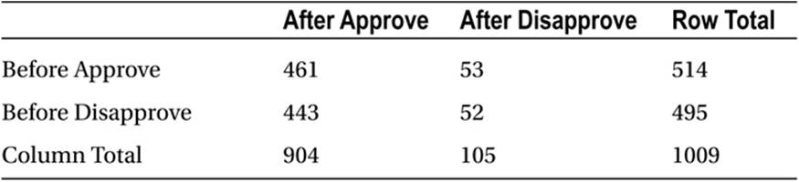
> BushApproval <- matrix(c(461,53,443,52),ncol = 2)
> BushApproval
[,1] [,2]
[1,] 461 443
[2,] 53 52
> mcnemar.test(BushApproval)

McNemar's Chi-squared test with continuity correction

data: BushApproval
McNemar's chi-squared = 305.0827, df = 1, p-value < 2.2e-16

We reach the rather obvious conclusion (which was supported by the Gallup polls in 2001) that Mr. Bush’s approval ratings increased significantly after 9/11.

The McNemar test is effective for tables in which b + c > 25. When b + c < 25, a binomial test can be used to determine the exact probability that b = c.

Recipe 10-3. Two-Sample Tests for Independent Means, Ranks, and Proportions

Problem

The use of independent samples to determine the effectiveness of some treatment or manipulation is common in research. The independent-samples t test applies when the dependent variable is interval or ratio in nature. We can use either the t test assuming equal variances in the population or the test assuming unequal variances. With ordinal data, the nonparametric alternative to the t test is the Mann-Whitney U test. We can use chi-square or z tests to compare independent proportions.

Solution

Parametric tests such as the t test and the analysis of variance (ANOVA) assume the data are interval or ratio, that the data are sampled from a normally distributed population, and that the variances of the groups being compared are equal in the population. To the extent that these assumptions are met, the standard hypothesis tests are effective. The central limit theorem allows us to relax the assumption of normality of the population distribution, as the sampling distribution of means converges on a normal distribution as the sample size increases, regardless of the shape of the parent population.

The traditional alternative to parametric tests when distributional assumptions are violated, as we have discussed and illustrated, is the use of distribution-free or nonparametric tests. However, the independent-samples t test assuming unequal variances is often a preferable alternative. InChapter 12, you will learn additional alternatives, most of which have been developed in the past 50 years, for dealing with data that are not normally distributed.

A two-sample z test is applicable when the population standard deviations are known or when the samples are large. As with the one-sample test, the two-sample z test is not built into base R. As mentioned previously, both one-sample and two-sample z tests are available in the BSDApackage. The z.test function in BSDA is quite flexible. Here is the one-sample z test output for our x array, and the results are identical to those from the z.test function we wrote earlier in Recipe 10-1.

> install.packages("BSDA")
> library(BSDA)
Loading required package: e1071
Loading required package: lattice

Attaching package: 'BSDA'

The following object is masked from 'package:datasets':

Orange

> z.test(x, mu = 70, sigma.x = 11)

One-sample z-Test

data: x
z = -1.8982, p-value = 0.05767
alternative hypothesis: true mean is not equal to 70
95 percent confidence interval:
61.51208 70.13592
sample estimates:
mean of x
65.824

A two-sample z test can be conducted using either known (unlikely) values for the population standard deviations or using the sample standard deviations (more likely) as estimates of the population parameters. The two-sample z test will produce identical test statistics as those of the independent-samples t test when the sample standard deviations are used, as the following output illustrates. See that the Welch t test adjusts the degrees of freedom to compensate for unequal variances. The data for x and y are as follows. Assume they represent the hypothetical scores of two different classes on a statistics course final.

> x
[1] 60.2 64.4 64.8 65.6 63.7 68.0 85.7 58.2 53.1 55.0 72.3 50.2 78.5 67.1 79.2
[16] 72.1 59.2 50.6 77.8 56.3 64.0 76.8 68.2 75.0 59.6
> y
[1] 84.5 89.7 74.0 90.4 84.9 99.6 90.0 94.2 91.2 95.2 91.4 79.0 75.9 77.9 90.9
[16] 79.7 85.6 85.2 91.0 79.8 82.5 80.7 86.4 81.2 94.1

> z.test(x, y, sigma.x = sd(x), sigma.y = sd(y))

Two-sample z-Test

data: x and y
z = -8.7317, p-value < 2.2e-16
alternative hypothesis: true difference in means is not equal to 0
95 percent confidence interval:
-24.94971 -15.80229
sample estimates:
mean of x mean of y
65.824 86.200

> t.test(x, y)

Welch Two Sample t-test

data: x and y
t = -8.7317, df = 42.768, p-value = 4.686e-11
alternative hypothesis: true difference in means is not equal to 0
95 percent confidence interval:
-25.08283 -15.66917
sample estimates:
mean of x mean of y
65.824 86.200

When the assumption of homogeneity of variance is justified, the independent-samples test assuming equal variances in the population is slightly more powerful than the Welch test. Let us compare the two tests. To conduct the pooled-variance t test, set the var.equal argument to T orTRUE. The value of t is the same for both tests, but the p values, degrees of freedom, and confidence intervals are slightly different. For the pooled-variance t test, the degrees of freedom are n₁ + n₂ – 2.

> t.test(x, y, var.equal = T)

Two Sample t-test

data: x and y
t = -8.7317, df = 48, p-value = 1.766e-11
alternative hypothesis: true difference in means is not equal to 0
95 percent confidence interval:
-25.06795 -15.68405
sample estimates:
mean of x mean of y
65.824 86.200

The wilcox.test function can be used to conduct an independent-groups nonparametric test. This test is commonly known and taught as the Mann-Whitney U test, but technically would be better labelled the Wilcoxon-Mann-Whitney sum of ranks test. To conduct the Mann-Whitney test, use the following syntax. We will continue with our example of the x and y vectors we worked with earlier. The Mann-Whitney test is often described as a test comparing the medians of the two groups, but it is really testing the locations of the two distributions. We see that when the data are converted to ranks, the difference is still significant.

> wilcox.test(x, y)

Wilcoxon rank sum test

data: x and y
W = 33, p-value = 8.5e-10
alternative hypothesis: true location shift is not equal to 0

Comparing two independent proportions can be accomplished by a z test or by a chi-square test, as we have discussed previously. Let us compare the two sample proportions and where x_i and n_i represents the counts of the occurrences and the samples size for sample i. A two-sample z test for proportions is calculated as follows:

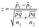
where is the pooled sample proportion, , and = 1 – .

As we have discussed, the square of the z statistic calculated by use of the preceding formula is distributed as chi-square with 1 degree of freedom. Let us do a one-tailed test with the following data to determine if airbags in automobiles save lives. The hypothetical data are as follows (seeTable 10-4).

Table 10-4. Hypothetical Airbag Data

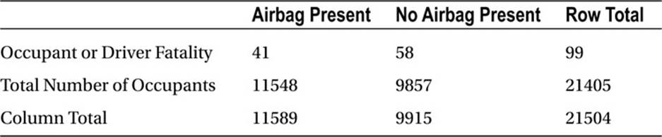
Either the chisq.test or the prop.test function can be used to test the hypothesis that the proportions are equal against the alternative that they are unequal. First, however, for instructive purposes, let us calculate the value of z using the formula shown earlier. We can write a reusable function as follows, passing the arguments x₁, x₂, n₁, and n₂, which are the number of “successes” and the column totals in Table 10-4.

z.prop <- function(x1, x2, n1, n2) {
p1 <- x1/n1
p2 <- x2/n2
p_bar <- (x1+x2)/(n1+n2)
q_bar <- 1-p_bar
pq <- p_bar * q_bar
z <- (p1 - p2)/sqrt((pq/n1)+(pq/n2))
return(z)
}
> z.prop(41,58,11589,9915)
[1] -2.496433

Now, for the sake of comparison, run the same test using the prop.test function in R. See that the square of z obtained by our function equals the uncorrected value of chi-square from the prop.test function.

> prop.test(x = c(41,58), n = c(11589, 9915), correct = FALSE)

2-sample test for equality of proportions without continuity
correction

data: c(41, 58) out of c(11589, 9915)
X-squared = 6.2322, df = 1, p-value = 0.01254
alternative hypothesis: two.sided
95 percent confidence interval:
-0.0041616709 -0.0004620991
sample estimates:
prop 1 prop 2
0.003537838 0.005849723

Recipe 10-4. Tests for Three or More Means

Problem

In many research studies, there are three or more means to compare. Although it is tempting to perform multiple t tests to test for mean differences, this results in a compounding Type I error. As a result, we are much more likely to reject a true null hypothesis than we would be for a single test at the same nominal alpha level. If each of the c tests is conducted with the same nominal alpha level, the actual Type I error rate compounds as follows:

The analysis of variance (ANOVA) controls the overall rate of a Type I error to no more than alpha, allowing us to determine if there are mean differences among two or more samples without inflating the probability of a Type I error.

Solution

To illustrate, with six means, there are ₆C₂ = 15 pairwise comparisons possible. Thus, the overall Type I error rate would be 1 – .95¹⁵ = .54, which is clearly far too high. R. A. Fisher developed the ANOVA to perform a single overall test with a controlled Type I error rate. If the overall test is significant, at least one pair of means is significantly different, and depending on the circumstances, one might conduct post hoc comparisons at a controlled Type I error rate to determine which means differ.

The one-way ANOVA compares means from independent samples. This test is a direct extension of the independent-samples t test, and produces identical results to the t test when two samples are compared. The repeated-measures ANOVA compares two or more means for the same subjects under different conditions or at different points in time. The repeated-measures ANOVA is a direct extension of the paired-samples t test. It is also possible to have multiple factors in an ANOVA. We will discuss the simplest of these cases, a balanced factorial design with two factors.

The parametric ANOVA assumes that the data are at least interval, that the measurements within a group are independent, and that the variances of the groups are equal in the population. When these assumptions are violated, the nonparametric alternatives to the one-way ANOVA and repeated-measures ANOVA are the Kruskal-Wallis analysis of variance for ranks and the Friedman test, respectively.

The aov and anova functions are part of base R. The ez package provides the ezANOVA function, which makes it easier to do between-groups and within-subjects ANOVAs, as well as mixed-model designs. Let us start with the one-way case. This is called a between-groups designbecause the groups are independent. As with the independent-samples t test, there is no requirement that the sample sizes must be equal for the one-way ANOVA. The overall F statistic is calculated as the ratio of the between-groups variance to the within-groups (error) variance. If the null hypothesis that the means are equal is true, the F ratio will be very close to 1. As the between-groups (treatment) variance becomes larger, the F ratio increases in value. We will begin our discussion with one-way tests for means and ranks.

One-Way Tests

The following data are from a study conducted at the University of Melbourne. The pain tolerance threshold was calculated for adult men and women with different hair colors. The higher the pain number, the greater the person’s tolerance for pain. Side-by-side boxplots are helpful to visualize the data. We see an obvious connection between hair color and pain thresholds. People with light blond hair are more pain tolerant than others. We will test the significance of this effect with a one-way ANOVA. The qplot function in ggplot2 produces the side-by-side boxplots (see Figure 10-3).

> hair
color pain
1 LightBlond 62
2 LightBlond 60
3 LightBlond 71
4 LightBlond 55
5 LightBlond 48
6 DarkBlond 63
7 DarkBlond 57
8 DarkBlond 52
9 DarkBlond 41
10 DarkBlond 43
11 LightBrunette 42
12 LightBrunette 50
13 LightBrunette 41
14 LightBrunette 37
15 DarkBrunette 32
16 DarkBrunette 39
17 DarkBrunette 51
18 DarkBrunette 30
19 DarkBrunette 35

> install.packages("ggplot2")
> library(ggplot2)
> qplot(factor(color), pain, data = hair, geom = "boxplot")

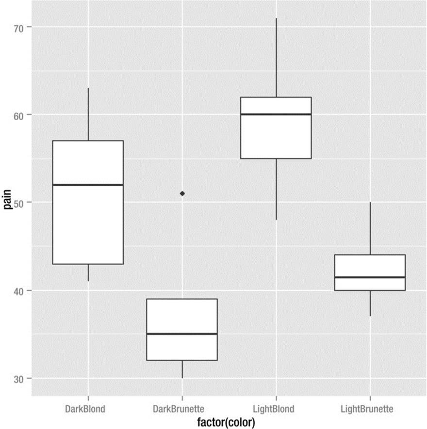
Figure 10-3. Pain threshold by hair color

Using the aov function, we see that the pain thresholds are statistically significantly different, though as yet we are not sure which means differ from one another. A popular post hoc test to compare pairs of means is the Tukey HSD (honestly significant difference) test, which is built into the base version of R as the function TukeyHSD. There are many other post hoc procedures, including Bonferroni corrections, the Scheffe test, and the Fisher LSD (least significant difference) criterion. First, examine the ANOVA summary table, and then the results of the Tukey HSD test, which shows that people with light blond hair have significantly higher pain thresholds than light and dark brunettes, but that light and dark blondes do not differ significantly.

> summary(model <- aov(pain ~ color, data = hair))
Df Sum Sq Mean Sq F value Pr(>F)
color 3 1361 453.6 6.791 0.00411 **
Residuals 15 1002 66.8
---
Signif. codes: 0 '***' 0.001 '**' 0.01 '*' 0.05 '.' 0.1 ' ' 1
> TukeyHSD(model)
Tukey multiple comparisons of means
95% family-wise confidence level

Fit: aov(formula = pain ~ color, data = hair)

$color
diff lwr upr p adj
DarkBrunette-DarkBlond -13.8 -28.696741 1.0967407 0.0740679
LightBlond-DarkBlond 8.0 -6.896741 22.8967407 0.4355768
LightBrunette-DarkBlond -8.7 -24.500380 7.1003795 0.4147283
LightBlond-DarkBrunette 21.8 6.903259 36.6967407 0.0037079
LightBrunette-DarkBrunette 5.1 -10.700380 20.9003795 0.7893211
LightBrunette-LightBlond -16.7 -32.500380 -0.8996205 0.0366467

The pain data do not appear to have equal variances, as the boxplots in Figure 10-3 imply. The car (Companion to Applied Regression) package provides several tests of homogeneity of variance, including the Levene test, which is used by SPSS as well. Let us determine whether the variances differ significantly. First, we will use the aggregate function to show the variances for the four groups, and then we will conduct the Levene test. The lack of significance for the Levene test is a function of the small sample sizes.

> aggregate(pain ~ color, data = hair, var)
color pain
1 DarkBlond 86.20000
2 DarkBrunette 69.30000
3 LightBlond 72.70000
4 LightBrunette 29.66667
> > install.packages("car")
> library(car)
> leveneTest(pain ~ color, data = hair)
Levene's Test for Homogeneity of Variance (center = median)
Df F value Pr(>F)
group 3 0.3927 0.76
15

Just as the independent-samples t test provides the options for assuming equal or unequal variances, the oneway.test function in R provides a Welch-adjusted F test that does not assume equality of variance. The results are similar to those of the standard ANOVA, which assumes equality of variance, but as with the t test, the values of p and the degrees of freedom are different for the two tests.

> oneway.test(pain ~ color, data = hair)

One-way analysis of means (not assuming equal variances)

data: pain and color
F = 5.8901, num df = 3.00, denom df = 8.33, p-value = 0.01881

When the assumptions of normality or equality of variance are violated, we can perform a Kruskal-Wallis analysis of variance by ranks using the kruskal.test function in base R. This test makes no assumptions of equality of variance or normality of distribution. It determines whether the distributions have the same shape, and is not a test of the equality of medians, though some statistics authors claim it is. The test statistic for the Kruskal-Wallis test is called H, and it is distributed as chi-square when the null hypothesis is true.

> kruskal.test(hair$pain, hair$color)

Kruskal-Wallis rank sum test

data: hair$pain and hair$color
Kruskal-Wallis chi-squared = 10.5886, df = 3, p-value = 0.01417

Two-Way Tests for Means

The two-way ANOVA adds a second factor, so that the design now incorporates a dependent variable and two factors, each of which has at least two levels. Thus the most basic two-way design will have four group means to compare. We will consider only the simple case of a balanced factorial design with equal numbers of observations per cell. With the two-way ANOVA, you can test for main effects for each of the factors and for the possibility of an interaction between them. From a research perspective, two-way ANOVA is efficient, because each subject is exposed to a combination of treatments (factors). Additionally, interactions are often of interest because they show us the limits or boundaries of the treatment conditions. Although higher-order and mixed-model ANOVAs are also possible, the interpretation of the results becomes more difficult as the design becomes more complex.

The two-way ANOVA can be conceptualized as a table with rows and columns. Let the rows represent Factor A, and the columns represent Factor B. In a balanced factorial design, each cell represents an independent group, and all groups have equal sample sizes. Post hoc comparisons are not necessary or possible when the design is a 2 × 2 factorial ANOVA, so we will illustrate with a 2 × 3 example. We consider only the fixed effects model here, but the interested reader should know that there are also random effects models in which the factor levels are assumed to be samples of some larger population rather than fixed in advance of the hypothesis tests. With the two-way ANOVA, the total sum of squares is partitioned into the effects due to Factor A, those due to Factor B, those due to the interaction of Factors A and B, and an error or residual term. Thus we have three null hypotheses in the two-way ANOVA, one for each main effect, and one for the interaction.

Assume we have data representing the job satisfaction scores for junior accountants after one year on their first job. The factors are investment in the job (high, medium, or low) and quality of alternatives (high or low). High quality alternatives represent attractive job opportunities with other employers. Although these data are fabricated, they are consistent with those presented by Rusbult and Farrell, the creators of the investment model,² which has been validated both in the workplace and in the context of romantic relationships. Assume we have a total of 60 subjects, so the two-way table has 10 observations per cell. For this example, let’s use the ezANOVA function in the ez package. The data are as follows:

> head(jobSat)
subject satisf alternatives investment
1 1 52 low low
2 2 42 low low
3 3 63 low low
4 4 48 low low
5 5 51 low low
6 6 55 low low
> tail(jobSat)
subject satisf alternatives investment
55 55 87 high high
56 56 80 high high
57 57 88 high high
58 58 79 high high
59 59 83 high high
60 60 80 high high

The output from the ezANOVA function shows that there is a significant main effect for investment and a significant interaction, but that the main effect for alternatives is not significant. When the interaction is significant, it is advisable to plot it in order to understand and interpret it before examining the main effects.

> install.packages("ez")
> library(ez)
> ezANOVA(data = jobSat, dv = satisf, wid = subject, between = .(alternatives, investment))
Warning: Converting "subject" to factor for ANOVA.
$ANOVA
Effect DFn DFd F p p<.05 ges
1 alternatives 1 54 0.8413829 3.630803e-01 0.01534212
2 investment 2 54 307.6647028 3.036366e-30 * 0.91932224
3 alternatives:investment 2 54 29.4058656 2.296500e-09 * 0.52132638

$`Levene's Test for Homogeneity of Variance`
DFn DFd SSn SSd F p p<.05
1 5 54 68.13333 519.3 1.416984 0.2329502

The Levene test reveals that the variances can be assumed to be homogeneous. The interaction plot can be generated by use of the interaction.plot function (see Figure 10-4).

> with(jobSat, interaction.plot(alternatives, investment, satisf, mean))

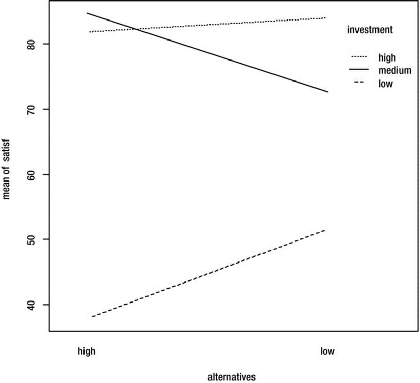
Figure 10-4. Interaction plot

Cautious interpretation of the main effect for investment indicates that for those who have made medium or high investment, job satisfaction is higher than for those who have made lower investment. However, the interaction effect shows that job satisfaction is lower for those who have medium investment if they have fewer job alternatives.

A little-known nonparametric alternative to the two-way ANOVA is the Scheirer-Ray-Hare (SRH) test. This test is not currently available in base or any contributed package I am able to locate. The SRH test is a direct extension of the Kruskal-Wallis analysis of variance by ranks to the two-way case. Not all statisticians agree that the SRH test is appropriate for ranked data. For example, Dr. Larry Toothaker of the University of Oklahoma discourages its use because it inflates the Type I error rate and does not test the interaction term correctly. A more effective nonparametric alternative to the factorial ANOVA is the aligned rank transform (ART) test. This test applies the traditional factorial ANOVA after the data have been “aligned” and ranked. A Windows program developed by Dr. Jacob Wobbrock of the University of Washington for aligning and ranking data can be found at http://depts.washington.edu/aimgroup/proj/art/.

Recipe 10-5. Repeated-Measures Designs

Problem

Repeated-measures designs involve measures of the same subjects either at different points in time or under different conditions. These are also known as within-subjects designs. One can test the subject effect and the treatment effect, though the subject effect is commonly not tested. In this design, each subject serves as its own control, and individual differences are allocated to systematic variation rather than to error. As a result, the error variation is reduced accordingly, and the tests of treatment effects are generally more powerful in repeated-measures designs than in between-groups designs.

Solution

We will consider the repeated measures design and illustrate its power relative to the one-way between-groups ANOVA. Then we will discuss the Friedman test as a nonparametric alternative to the repeated-measures ANOVA.

The repeated-measures design can be thought of as a special case of the two-way ANOVA with one observation per cell. With one observation, there is no within-cell variance, but the cells for a single subject can be compared to the overall subject total. The sums of squares for treatments and for subjects are calculated as in the one-way ANOVA. The absence of within-cell variation means there is no ability to test an interaction effect, and the subject x treatment interaction mean square is used as the error term in repeated-measures ANOVA. The repeated-measures ANOVA also applies to experiments in which randomized blocks are used to control for “nuisance” factors.

To illustrate the power of the repeated-measures design relative to the between-groups design, let us consider the following example modified from Welkowitz, Cohen, and Ewen (2006). In this hypothetical example, subjects listened to classical music while performing a spatial ability test. The study was designed to test the so-called “Mozart” effect in which listening to classical music—especially that of Mozart—is believed to improve spatial reasoning, at least momentarily. We will first treat the data as a between-groups design and then run a repeated-measures analysis assuming that each subject listened to all five composers. We see that the one-way ANOVA is not significant:

> music <- read.csv("music.csv")
> head(music)
Person Subject Composer Score
1 1 1 Mozart 16
2 2 2 Mozart 16
3 3 3 Mozart 14
4 4 4 Mozart 13
5 5 5 Mozart 12
6 6 1 Chopin 16
> tail(music)
Person Subject Composer Score
20 20 5 Schubert 12
21 21 1 Beethoven 14
22 22 2 Beethoven 13
23 23 3 Beethoven 13
24 24 4 Beethoven 10
25 25 5 Beethoven 10
> factor(music$Composer)
[1] Mozart Mozart Mozart Mozart Mozart Chopin Chopin
[8] Chopin Chopin Chopin Bach Bach Bach Bach
[15] Bach Schubert Schubert Schubert Schubert Schubert Beethoven
[22] Beethoven Beethoven Beethoven Beethoven
Levels: Bach Beethoven Chopin Mozart Schubert
> between <- lm(Score ~ Composer, data = music)
> anova(between)
Analysis of Variance Table

Response: Score
Df Sum Sq Mean Sq F value Pr(>F)
Composer 4 14.4 3.60 0.8411 0.5154
Residuals 20 85.6 4.28

Now, let us recast the analysis as a repeated-measures ANOVA. We assume each person listened to all five composers and completed five parallel versions of the spatial ability test. To control for order and sequencing effects, let us further assume that each person listened to the five composers in random order, controlled by the computer. Although there are many different ways to run the repeated-measures ANOVA, one effective way is to use the ezANOVA function in the ez package.

> ezANOVA(data = music, dv = Score, wid = Subject, within = Composer)
Warning: Converting "Subject" to factor for ANOVA.
$ANOVA
Effect DFn DFd F p p<.05 ges
2 Composer 4 16 5.538462 0.005399203 * 0.144

$`Mauchly's Test for Sphericity`
Effect W p p<.05
2 Composer 0.591716 0.9989984

$`Sphericity Corrections`
Effect GGe p[GG] p[GG]<.05 HFe p[HF] p[HF]<.05
2 Composer 0.845 0.009177744 * 6.008065 0.005399203 *

The F ratio for the repeated-measures analysis is significant at p = .005. The repeated-measures ANOVA assumes sphericity, which is the assumption that the differences between the variances of the repeated measures are equal in the population. Unlike the homogeneity of variance assumption in one-way ANOVA, the sphericity assumption is more restrictive, and violations of it lead to substantial increases in Type I error. The Mauchly test confirms that we can assume the sphericity assumption was met in this case. In cases where the sphericity assumption is violated, the two common corrections are to multiply the degrees of freedom by a correction factor known as ε (Greek letter epsilon). The first method of calculating ε is known as the Greenhouse-Geisser (GGe), and the second is known as the Huyn-Feldt (HFe).

When the overall F ratio is significant, it is customary to employ post hoc tests to determine the patterns of significance in the repeated measures. The two most common approaches are to use the Tukey HSD test illustrated in Recipe 10-4 or to use Bonferroni-adjusted comparisons. Let us illustrate the use of the Bonferroni technique. Because there are ₅C₂= 10 pairs of means, the adjusted alpha level for the Bonferroni comparisons would be .05 / 10 = .005. The Bonferroni-adjusted comparisons reveal that only the comparison between Beethoven and Mozart is significant. Here are the means followed by the Bonferroni-adjusted pairwise t tests.

> aggregate(Score ~ Composer, data = music, mean)
Composer Score
1 Bach 12.4
2 Beethoven 12.0
3 Chopin 13.2
4 Mozart 14.2
5 Schubert 13.2

> with(music, pairwise.t.test(Score, Composer, p.adjust.method = "bonferroni", paired = T))

Pairwise comparisons using paired t tests

data: Score and Composer

Bach Beethoven Chopin Mozart
Beethoven 1.000 - - -
Chopin 1.000 1.000 - -
Mozart 0.213 0.042 0.890 -
Schubert 1.000 1.000 1.000 0.890

P value adjustment method: bonferroni

The Friedman test is a nonparametric alternative to the repeated-measures ANOVA. As with most other nonparametric tests, the dependent variable is converted to ranks. In the case of repeated-measures, the data are ranked for a given subject, and the ranks for the treatments across subjects are tested for significance. When the overall Friedman test is significant, the most common follow-up test is the use of multiple Wilcoxon signed rank tests. As with the parametric tests, it is important to recognize and control for the inflated Type I error resulting from multiple pairwise comparisons. Here is the Friedman test applied to the current data. For the sake of convenience, I transformed the data to a “wide” format and saved it as a matrix to simplify the application of the Friedman test. The test shows that there is an effect of the composer, just as the parametric test indicated.

> musicWide
Mozart Chopin Bach Schubert Beethoven
1 16 16 16 16 14
2 16 14 14 14 13
3 14 13 12 12 13
4 13 13 10 12 10
5 12 10 10 12 10
> musicWide <- as.matrix(musicWide)
> friedman.test(musicWide)

Friedman rank sum test

data: musicWide
Friedman chi-squared = 11.1169, df = 4, p-value = 0.02528

______________________

¹These data are loosely based on the Gallup poll results reported at http://www.gallup.com/poll/116500/presidential-approval-ratings-george-bush.aspx.

²See Rusbult, C. E., and Farrell, D. (1983). A longitudinal test of the investment model. The impact on job satisfaction, job commitment, and turnover of variations in reward, costs, alternatives, and investments. Journal of Applied Psychology, 68, 429–438.